
Lecture
In the implementation of mathematical models of electrical circuits, the problem of finding stationary solutions of systems of differential equations is one of the central ones. This is because stationary solutions describe steady-state conditions, which for electrical circuits are the ordinary operating states.
Stationary state in the theory of dynamical systems — is a state of a system or process in which the dynamics of the variables describing the behavior of the system or process, and called state variables, do not change over time (unlike a transient process). Synonyms: stationary solution, stationary regime, stationary motion, steady-state motions
Stationary motion is the limiting motion of a system, that is, the motion the system tends toward; moreover, a state of rest is also regarded as a special case of stationary motion. It is precisely the stationary motions of a system that are the most characteristic of the system's behavior over long periods of time.
It is customary to distinguish between a stable and an unstable stationary state.
Examples of stationary states include: a focus, a node, a saddle, and a limit cycle.
The solution of the system of differential equations satisfying the initial conditions X(t0)=Q,we shall denote byX(t, t0 , Q).
In this textbook we shall consider methods for finding stationary solutions of normal systems of first-order linear inhomogeneous differential equations with constant coefficients and an external periodic excitation.
The solution of such systems has the form
 (2.17)
where Xn(t) -is a stationary solution of the periodic type, representing a particular solution of the system of inhomogeneous differential equations.
The character of the particular solution of the system of linear inhomogeneous differential equations is determined by the character of the external excitation on the circuit.
Let the external excitation be periodic and have the form:
 (2.18)
In this case, the system of differential equations (2.17) can be represented in the form:
 (2.19)
where B0 -is the vector of external excitations corresponding to the termU0;
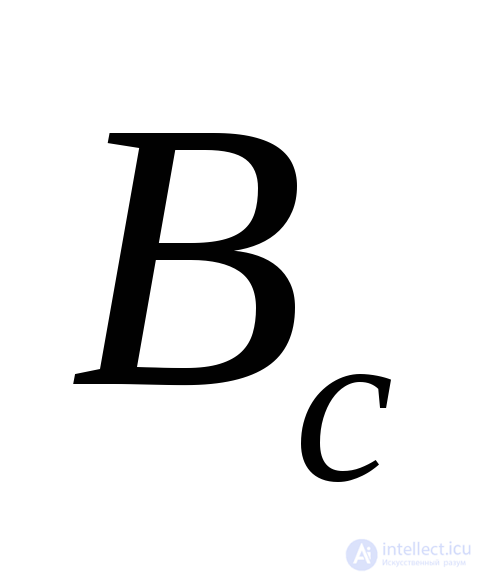 - is the vector of external excitations corresponding to the term
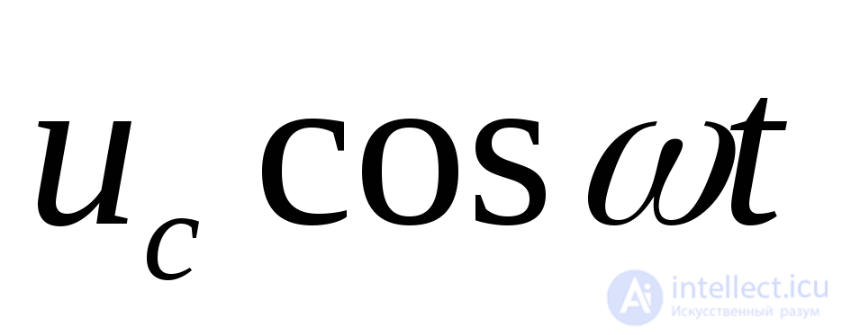 ;
; 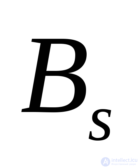 -is the vector of external excitations corresponding to the term
 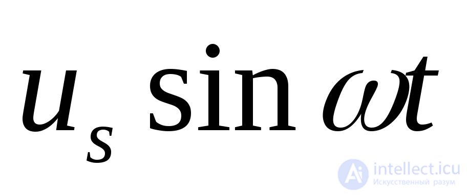 .
.
A particular solution of this system of equations has the form:
 (2.20)
where Do, Dc, Ds -are one-column matrices, which are determined by substituting (2.19) into (2.20). Omitting the intermediate transformations, we write:
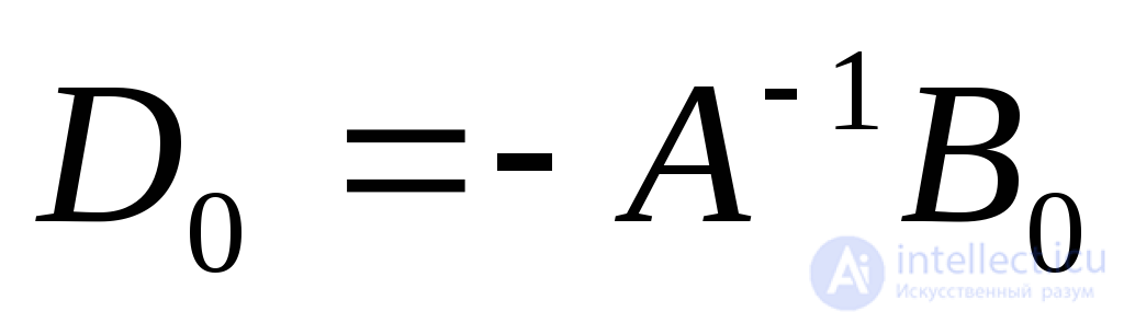
 (2.21)

where E -is the identity matrix.
The direct method for finding stationary periodic solutions of systems of linear differential equations is based on the possibility of writing such a solution in explicit form:
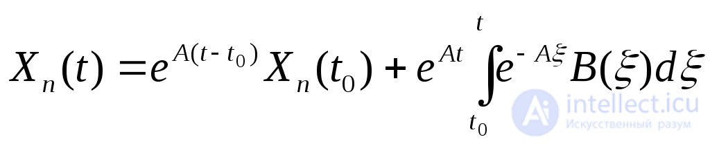
or  , (2.22)
where 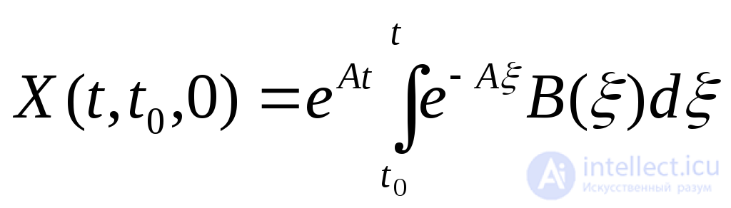 - is the solution of the Cauchy problem with zero initial conditions
The essence of the direct method reduces to determining the vector Xn(t0)of initial conditions for the periodic solution. Using the periodicity condition

from (2.22) we find
 (2.23)
Since the solution is periodic with period T,it suffices to choose the initial moment of timet0 within the interval[0,T],that is 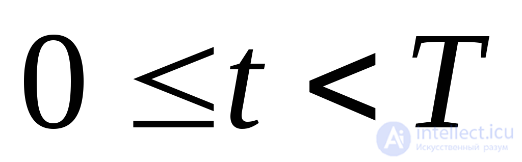 .Without loss of generality, we shall choose the initial moment of timet0 = 0,in which case the expression for the initial conditions of the periodic solution (2.23) takes the form
 (2.24)
where X(T,0) - is the solution of the Cauchy problem with initial conditionsX(0) = O
Thus, in order to find the periodic solution by the direct method, the following steps must be carried out:
solve the Cauchy problem over one period with zero initial conditions using one of the numerical methods; as a result the vector X(T,0); is determined
compute the matrix exponential eAT;
determine the vector of initial conditions of the periodic solution Xn(0)using formula (2.24);
solve the Cauchy problem for the original system of differential equations over one period with initial conditions X(0)=Xn(0).
Fig. 2.3 shows the block diagram for finding the vector Xn(0)of initial conditions of the periodic solution by the direct method.
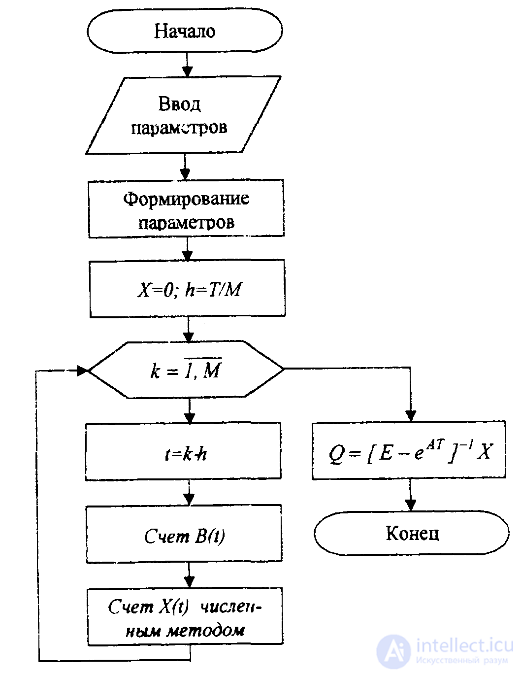
Fig 2.3
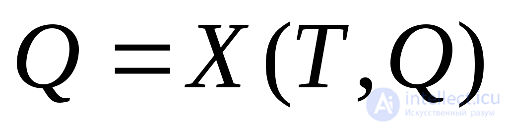
Assuming the initial moment of time tn=0and taking into account the periodicity condition, the search for the periodic solution of the system of differential equations can be reduced to solving a system of transcendental equations with respect to the vector of initial conditionsQ
 (2.25)
The simplest and most natural way of solving system (2.25) is the simple iteration method:
 (2.15) (2.26)
where the initial approximation vector Q(0)is specified arbitrarily. Each successive approximationQ(s+1)is found by solving the Cauchy problem on the interval(0, T)with the initial condition given by the previous approximationQ(s). On the other hand, taking into account the periodicity of the right-hand side of the system of differential equations,Q(s+1)is determined by solving the Cauchy problem on the interval with the conditionX(sT)=QS,that is, carrying out the iterative process (2.15) is equivalent to solving the Cauchy problem with the initial condition given by the vectorQ(0), over a time interval whose duration is determined by the convergence conditions. For this reason the method of finding the vector of initial conditions of the periodic solution by numerical scheme (2.26) is also called the settling method (method of establishment), or finding the periodic solution via the transient process.
The choice of the termination criterion for the iterative process (2.26) depends on the choice of norm in the vector space.
If the vector norm is defined as  , then the satisfaction of the following inequality is chosen as the convergence criterion:
 (2.27)
If the following is adopted as the vector norm, then the criterion 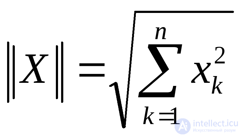 for terminating the iterative process will be the inequality:
 (2.28)
In inequalities (2.27) and (2.28) the quantity 8determines the relative difference between two neighbouring approximations, that is, it characterises the relative accuracy of computing the vector of initial conditions of the periodic solution. A block diagram of the algorithm for finding the periodic solution by the settling method is shown in Fig. 2.4.
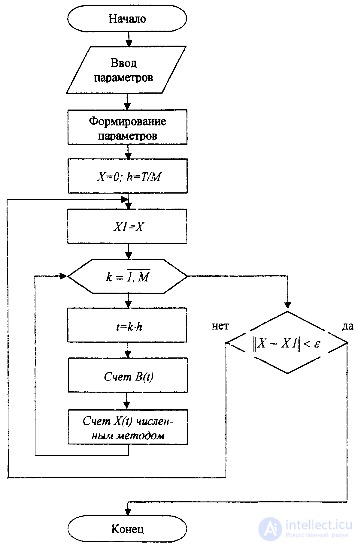
Fig. 2.4

Comments