
Lecture
The Lotka–Volterra equations , also known as the Lotka–Volterra predator–prey model , are a pair of first-order nonlinear differential equations often used to describe the dynamics of biological systems in which two species interact: one as a predator, and the other as prey. The population sizes change over time according to this pair of equations: ,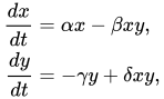
where
 and
and  represent the instantaneous growth rates of the two populations;
The solution of the differential equations is deterministic and continuous . This, in turn, means that the generations of predator and prey are continually overlapping.
The system of Lotka-Volterra equations is an example of a Kolmogorov population model (not to be confused with the better-known Kolmogorov equations ) , which represents a more general framework allowing the modelling of the dynamics of ecological systems with predator-prey interactions, competition , diseases and mutualism .
The prey are assumed to have an unlimited food supply and to reproduce exponentially unless subject to predation; this exponential growth is represented in the equation above by the term αx . The rate of predation on the prey is assumed to be proportional to the rate at which predators and prey meet; this is represented above by the term βxy . If x or y is zero, there can be no predation. With these two terms, the equation above for the prey can be interpreted as follows: the rate of change of the prey population is given by its own growth rate minus the rate at which it is preyed upon.
The term δxy represents the growth of the predator population. (Note the similarity to the predation rate; however, a different constant is used, since the predator population's growth rate is not necessarily equal to the rate at which it consumes prey). The term γy represents the rate of decline of the predator population due to natural death or emigration; in the absence of prey this results in exponential decay. Thus, the equation shows that the rate of change of the predator population depends on the rate at which it consumes prey, minus its own mortality rate.
The Lotka-Volterra predator-prey model makes a number of assumptions about the environment and the biology of the predator and prey populations:
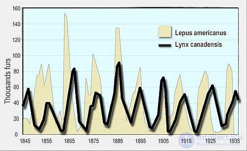
The quantity of snowshoe hare pelts (yellow, in the background) and Canada lynx pelts (black line, in the foreground) sold to the «Hudson's Bay» company . Canada lynxes feed on snowshoe hares.
None of the above assumptions is likely to hold for natural populations. Nevertheless, the Lotka-Volterra model demonstrates two important properties of predator and prey populations, and these properties often carry over to variants of the model in which these assumptions are relaxed:
First, the dynamics of predator and prey populations tend towards oscillation. Oscillations in the numbers of predators and prey have been observed in natural populations, for example, the lynx and snowshoe hare data of the Hudson's Bay Company and the populations of moose and wolves on Isle Royale National Park .
Second, the equilibrium of the population in this model has the property that the equilibrium prey density (given by the formula)  ) depends on the predator parameters and the equilibrium predator density (given by the formula
  ) on the prey parameters. This leads, as a consequence, to an increase in, for example, the prey growth rate.α This leads to an increase in the equilibrium predator density, but not the equilibrium prey density. An improvement in conditions for the prey benefits the predator, not the prey (this is related to the pesticide paradox and the paradox of enrichment ). A demonstration of this phenomenon is the increase in the percentage of predatory fish caught during the years of the First World War (1914–1918), when the growth rate of prey increased due to the reduction in fishing effort.
Another example — experimental iron fertilisation of the ocean . In several experiments, large quantities of iron salts were dissolved in the ocean. It was expected that iron, being the limiting nutrient for phytoplankton, would stimulate phytoplankton growth and absorb carbon dioxide from the atmosphere. The addition of iron usually results in a short-lived phytoplankton bloom, which is quickly consumed by other organisms (such as small fish or zooplankton ) and limits the effect of enrichment mainly through an increase in predator density, which, in turn, limits carbon uptake . This corresponds to the predictions of the equilibrium population densities of the Lotka-Volterra predator-prey model and is a feature that persists even in more complex models in which the restrictive assumptions of the simple model are relaxed.
The Lotka-Volterra model has additional applications in fields such as economics and marketing . It can be used to describe the dynamics of a market with several competitors, complementary platforms and products, the sharing economy, and much more. There are situations in which one competitor displaces other competitors from the market, and other situations in which the market reaches an equilibrium in which each firm stabilises its market share. It is also possible to describe situations in which an industry undergoes cyclical changes or chaotic situations without equilibrium, with frequent and unpredictable changes.
In economics, the Phillips curve , which shows the statistical relationship between unemployment and the rate of change of nominal wages, has been linked to the Goodwin model . This model reinterprets the dynamics of biological predator-prey interaction described by the Lotka-Volterra model in economic terms. The way the two species interact in this model led Goodwin to draw parallels with Marxist class conflict . A generalisation of the Kolmogorov predator-prey model, together with further development of the Goodwin model, extended these ideas.
The Lotka-Volterra predator-prey model was first proposed by Alfred J. Lotka in the theory of autocatalytic chemical reactions in 1910. In essence, this was the logistic equation , originally derived by Pierre Francois Verhulst . In 1920 Lotka extended the model, via Andrey Kolmogorov , to «organic systems», using as an example a plant species and a herbivore species , and in 1925 he used the equations to analyse predator-prey interactions in his book on biomathematics . The same set of equations was published in 1926 by Vito Volterra , a mathematician and physicist who had become interested in mathematical biology . Volterra's research was inspired by his interaction with the marine biologist Umberto D'Ancona , who at the time was courting his daughter and later became his son-in-law. D'Ancona studied fish catches in the Adriatic Sea and noticed that the percentage of predatory fish caught increased during the years of the First World War (1914–1918). This puzzled him, since fishing effort had been significantly reduced during the war years, and, since predatory fish were the preferred catch, one would intuitively expect an increase in the percentage of predatory fish. Volterra developed his model to explain D'Ancona's observation and did so independently of Alfred Lotka. He pointed to Lotka's earlier work in his publication, after which the model became known as the «Lotka-Volterra model».
Later the model was extended to include density-dependent prey growth and a functional response in the form developed by C. S. Holling ; a model that became known as the Rosenzweig-MacArthur model. Both the Lotka-Volterra model and the Rosenzweig-MacArthur model have been used to explain the dynamics of natural predator and prey populations.
In the late 1980s an alternative to the Lotka-Volterra predator-prey model (and its generalisations dependent on total prey) appeared — a ratio-dependent model, or the Arditi-Ginzburg model . [ 23 ] The validity of prey-dependent or ratio-dependent models has been widely debated.
The Lotka-Volterra equations have a long history of application in economic theory ; their first application is usually attributed to Richard Goodwin in 1965 or 1967 .
The equations have periodic solutions. These solutions do not have a simple expression in terms of the usual trigonometric functions , although they are quite amenable to computation.
If none of the non-negative parameters α , β , γ , δ is zero, three of them can be absorbed into the normalisation of the variables, leaving only one parameter: since the first equation is homogeneous in x , and the second in y , the parameters β / α and δ / γ can be absorbed into the normalisation of y and x respectively, and γ — into the normalisation of t , so that only α / γ remains arbitrary. This is the only parameter that affects the character of the solutions.
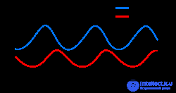
Dynamics of the numbers of prey and predators over time
Linearisation of the equations gives a solution analogous to simple harmonic motion , where the predator population lags behind the prey population by 90° in the cycle.
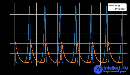
Let us set aside the problem of the population dynamics of rabbits and foxes.
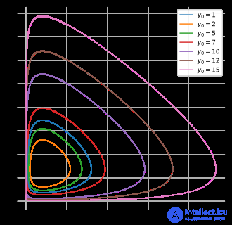
Phase-space diagram for the «predator-prey» problem under various initial conditions for the predator population.
Suppose there are two species of animals: the rabbit (prey) and the fox (predator). If the initial density is 10 rabbits and 10 foxes per square kilometre, one can plot the change in the numbers of these two species over time, given that the growth and mortality rates for rabbits are 1.1 and 0.4, and for foxes — 0.1 and 0.4 respectively. The choice of the time interval is arbitrary.
The solutions can also be plotted parametrically as orbits in phase space , without representing time, but with one axis representing the number of prey and the other axis representing the density of predators at all points in time.
This corresponds to eliminating time from the two differential equations given above, which results in a single differential equation.
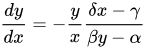
The equation relates the variables x (prey) and y (predator). The solutions of this equation are closed curves. It is amenable to the method of separation of variables : integrating
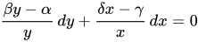
leads to the implicit relation
V=δx−γln(x)+βy−αln(y),
where V — is a constant, dependent on the initial conditions and preserved along each curve.
Note: These graphs illustrate a serious potential limitation of the model's application as a biological model: with this particular choice of parameters, in each cycle the rabbit population is reduced to extremely small values, but then recovers (whereas the fox population remains significant at the lowest rabbit density). However, under real conditions, random fluctuations in the discrete number of individuals could lead to the actual extinction of the rabbits, and consequently of the foxes as well. This modelling problem has been named the «atto-fox problem», where an atto-fox — is a notional 10⁻¹⁸ foxes . A density of 10⁻¹⁸ foxes per square kilometre corresponds on average to approximately 5×10⁻¹⁰ foxes over the surface of the Earth, which in practice means the extinction of foxes.
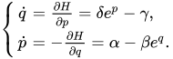
Since the quantity  is conserved in time, it plays the role of the Hamiltonian function of the system. To verify this, we can define the Poisson bracket as follows
  Then Hamilton's equations take the following form :
 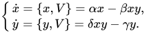 The variables x
 and y
and y are not canonical, since
  However, using the transformations
  and
and  we arrive at the canonical form of Hamilton's equations, involving the Hamiltonian.
  :
:  The Poisson bracket for the canonical variables (q,p)
 now takes the standard form
  .
.
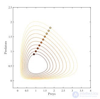
Another example covers:
α = 2/3 , β = 4/3 , γ = 1 = δ . Suppose that x and y are measured in thousands. The circles represent initial conditions for prey and predator from x = y = 0.9 to 1.8 in steps of 0.1. The fixed point is located at (1, 1/2).
In the model system, predators thrive when prey is abundant, but eventually their numbers exceed the capacity of the food supply, and their numbers decline. As the number of predators decreases, the prey population increases again. This dynamic continues in a cycle of population growth and decline .
In the model, population equilibrium is reached when neither population level is changing, that is, when both derivatives are equal to 

The system of equations above gives two solutions:  and
and 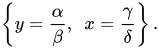
Consequently, there are two states of equilibrium.
The first solution effectively represents the extinction of both species. If the numbers of both populations are zero, they will remain at that level indefinitely. The second solution represents a fixed point at which both populations maintain their current, non-zero numbers and, in the simplified model, do so indefinitely. The population levels at which this equilibrium is reached depend on the chosen values of the parameters α , β , γ and δ .
The stability of the fixed point at the origin can be determined by performing a linearisation using partial derivatives .
The Jacobian matrix of the «predator-prey» model has the form: 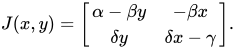 and is known as the community matrix .
Evaluated at the steady state (0, 0), the Jacobian matrix J takes the form J.( 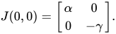
The eigenvalues of this matrix are 
In this model, α and γ are always greater than zero, and, consequently, the sign of the eigenvalues will always differ. Thus, the fixed point at the origin is a saddle point .
The instability of this fixed point is of major significance. If it were stable, non-zero populations might be attracted to it, and, consequently, the dynamics of the system could lead to the extinction of both species for many initial population levels. However, since the fixed point at the origin is a saddle point and, consequently, unstable, it follows that the extinction of both species is difficult to achieve in this model. (In fact, this could occur only if the prey were artificially completely exterminated, which would lead to the predators dying of starvation. If the predators were exterminated, the prey population would grow without bound in this simple model.) The prey and predator populations can approach zero by an infinitesimally small amount and still recover.
Evaluating J at the second fixed point gives 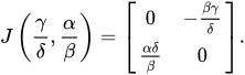
The eigenvalues of this matrix are 
Since the eigenvalues are purely imaginary and conjugate to one another, this fixed point must be either the centre of closed orbits in the local neighbourhood, or an attracting or repelling spiral. In conservative systems there must exist closed orbits in the local neighbourhood of fixed points that are at the minima and maxima of the conserved quantity. The conserved quantity, as shown above, has the form:  on the orbits. Thus, the orbits around the fixed point are closed and elliptical , so the solutions are periodic, oscillating on a small ellipse around the fixed point with frequency.
  and period
  .
.
As shown in the figure above, the circulating oscillations are closed orbits around the fixed point: the levels of predator and prey populations change cyclically and oscillate without decay around the fixed point at a specific frequency.ω=αγ .
.
The value of the constant of motion V , or, equivalently,  , can be found for closed orbits near the fixed point.
Increasing K brings the closed orbit closer to the fixed point. The largest value of the constant K is obtained by solving the optimisation problem. 
Thus, the maximum value of K is attained at the stationary (fixed) point.  and is equal to
 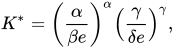 where e — is Euler's number .

Comments