
Lecture
Determining the velocity of a particle. The position of a particle at time t is given by its radius vector r ( t ); the derivative of the vector function r ( t ) is called the velocity of the particle:

Definition of momentum. The product
p = m v
of the mass of a particle and its velocity is called the momentum of the particle.
Newton's second law. Newton's second law states that the rate of change of the momentum of a particle is equal to the force F acting on the particle:
dp / dt = F.
Substituting for the momentum its expression, we obtain the familiar formula:
m dv / dt = F.
This vector equation is equivalent to three scalar equations:
m dvx / dt = Fx,
m dvy / dt = Fy,
m dvz / dt = Fz,
vx, vy, vz – the coordinates of the velocity vector v, Fx, Fy, Fz, - the coordinates of the force vector F.
Determining work. Suppose that at time t the radius vector of a particle equals r ( t ) and the force F ( t ) acts on it, t1 ≤ t ≤ t2. In displacing the particle, the force F did an amount of work A, equal to
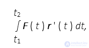
the integrand is equal to the scalar (dot) product of the force vector F ( t ) and the velocity vector r ' ( t ) (the scalar product of two vectors equals the sum of the products of their corresponding coordinates).
Motion of a particle in a uniform gravitational field. A particle (a point mass) falls vertically downward in an airless space under the action of a constant force of gravity. Let us choose a coordinate system such that the plane Oxy coincides with the surface of the Earth, the axis Oz is directed vertically upward, and the particle moves along the axis Oz. The force of gravity acting on the particle is proportional to its mass, the coefficient of proportionality being equal to the acceleration of free fall:
m dv / dt = - m g
(the 'minus' sign on the right-hand side indicates that the force of gravity is directed downward).
Fall of a ball. A ball moves along the vertical axis Oz under the action of a constant force of gravity; the air-resistance force is proportional to the velocity of the ball.
The ball is acted on by the force of the Earth's attraction, proportional to the mass of the particle, the coefficient of proportionality being equal to the acceleration of free fall:
Fgrav = - m g
(the 'minus' sign on the right-hand side indicates that the force of gravity is directed downward). The air-resistance force equals – k v:
Fres = - k v,
the minus sign indicates that the direction of the air-resistance force and the direction of the particle's velocity are opposite. The equation of motion of the ball:
m dv / dt = - k v – m g.
Directed segments. The values of many physical quantities cannot be represented by means of a single real number (a scalar). The displacement of a particle in space, the velocity of a particle, its acceleration, and a force are depicted in the form of directed segments (vectors) connecting two points of a line, a plane or space. In what follows, vector quantities are denoted by bold letters.
Coordinates of a directed segment. The coordinates of a directed segment are its projections onto the coordinate axes. A particular case of a directed segment is the radius vector of a point, which connects the origin of coordinates with that point. The coordinates of a point M coincide with the coordinates of its radius vector. To calculate the coordinates of a directed segment MN, one should subtract the corresponding coordinates of the start (point M ) from the coordinates of its end (point N );
Addition of directed segments and their multiplication by numbers. Directed segments are added according to the parallelogram rule or the triangle rule. When directed segments are added, their corresponding coordinates are added, and when a directed segment is multiplied by a number, each coordinate is multiplied by that number.
Distance between vectors. The distance between vectors a, b is denoted by the symbol | a – b |:
| a – b | = (( a1 – b1 )2 + ( a2 – b2 )2 + ... + ( an – bn )2 )1/2,
where (a1, a2, …, an) – the coordinates of vector a, and (b1, b2, …, bn) – coordinates of the vector b.
Definition of a function. A quantity y is called a function of a quantity x if to every value of x from some set X there is assigned, by a definite rule, a value y. The set X is called the domain of definition of the function, and the quantity x is called the independent variable (sometimes the argument) of the function y. The functional dependence between the quantities y and x is expressed as follows: y = f ( x ); the letter f in this equality denotes the rule that establishes the correspondence between x and y.
The exponential function. The base of the exponential function ex or exp ( x ) is Euler's number e = 2.71828… . All values of the exponential function are positive; it converts a sum into a product, and a difference – into a ratio:
exp ( x + y ) = exp ( x ) exp ( y ),
exp ( x – y ) = exp ( x ) / exp ( y ),
exp ( -x ) = 1 / exp ( x ),
exp ( 0 ) = 1.
Sine and cosine. The coordinates of a directed segment of length r, lying in the plane xOy and forming an angle φ with the axis Ox, are equal to ( r cos φ, r sin φ, 0 ). By the Pythagorean theorem
cos2 φ + sin2 φ = 1 (the fundamental trigonometric identity).
Scalar and vector functions. If all values of the quantity y are real numbers, then the function y = f ( x ) is said to be scalar. A vector function of dimension n is given by a set of n real (scalar) functions, which are called its coordinate functions.
Definition of a limit. A number b is called the limit of a (scalar) function f ( x ) as x tends to a, if for every positive number ε there can be found a positive number δ such that | f ( x ) – b | < ε, whenever x belongs to the domain of definition of the function f, | x - a | < δ and x is not equal to a. Thus, as x approaches a, f ( x ) approaches b. The limit of the function f ( x ) as x tends to a is denoted by the symbol
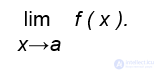
The limit of a vector function is defined analogously; in this case | f ( x ) – b | is the distance between the vectors f ( x ) and b.
Limits with infinitely distant elements. In many problems, alongside ordinary numbers, one must consider infinitely distant elements ∞, +∞, -∞. A number or vector b is called the limit of the function f ( x ) as x tends to +∞, if for every positive number ε there can be found a positive number d such that | f ( x ) – b | < ε, whenever x > d.
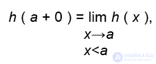
One-sided limits. The limit
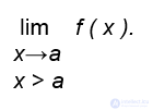 (respectively,
 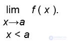 ) is called the one-sided limit of the function f ( x ) as x tends to a from the right (respectively, from the left) and is denoted by the symbol f ( a + 0 ) (respectively, f ( a – 0 )).
The Heaviside function. We denote the Heaviside function by the symbol χ ( x ): χ ( x ) = 1, when t > 0 and χ ( x ) = 0, when x ≤ 0;
χ ( x + 0 ) = 1,
χ ( x - 0 ) = χ ( 0) = 0.
Properties of limits. The limit of a constant function equals that constant. If, as x tends to a, the limits lim f (x ) and lim g (x ) exist, then the limit of the sum of the functions f (x ), g (x ) equals the sum of the limits of the terms, the limit of a product equals the product of the limits of the factors, and a constant factor may be taken outside the limit sign.
Continuous functions. A function f ( x ) is called continuous at a point a if it is defined at that point and lim f ( x ) = f ( a ) when x tends to a (a small increment of the argument corresponds to a small change in the function). If the domain of definition of a function is a numerical interval and the function is continuous at every point of that interval, then its graph can be drawn without lifting the pencil from the paper.
Continuity of elementary functions. Elementary functions (constant, power, exponential, trigonometric), as well as functions obtained from them by the operations of addition, subtraction, multiplication, division, substitution of a function in place of the argument of another function, and passage to the inverse function, are continuous at every point where they are defined. The Heaviside function has a discontinuity at zero.
Definition of the derivative. The derivative (scalar or vector) of a function f at a point x is called the limit of the ratio of the increment of the function to the increment of the argument at that point, as the increment of the argument tends to zero. This limit is denoted by the symbol f´ ( x ):

Computing the derivatives of a vector function. The coordinate functions of the derivative of a vector function equal the derivatives of the corresponding coordinate functions of the original vector function.
An example of computing derivatives. Let f ( x ) = x, g ( x ) = x2 , then
f´( x ) = lim ( ( x + Δx ) – x ) / Δx = lim Δx / Δx =1,
g´( x ) = lim ( ( x + Δx )2 – x2 ) / Δx = lim ( 2 x Δx + Δx2) / Δx = lim ( 2 x + Δx ) = 2 x
(Δx tends to 0).
Rules of differentiation
( f ( x ) + g ( x ))´ = f´( x ) + g´( x ),
( a f ( x ))´ = a f´( x )
(the derivative of a sum of functions equals the sum of their derivatives, a constant factor may be taken outside the sign of the derivative);
( f ( g ( x ) )´ = f´ ( g ( x ) ) g´ ( x )
(the derivative of a composition of functions), the expression ( f ( g ( x ) )´ on the left denotes the derivative of the function ( f ( g ( x ) ) at the point x, while the expression ( f' ( g ( x ) ) on the right denotes the derivative of the function f at the point g ( x )
Derivatives of elementary functions. The derivative of a constant function equals zero;
( x )´ = 1;
( xa )´ = a xa-1;
( exp ( x ))´ = exp ( x ).
The second-order derivative. If the function f has a derivative at every point located near the point x, then one can define the second-order derivative of the function f at the point x:
f΄΄( x ) = lim (( f´( x + Δx ) – f´( x ) ) / Δx )
Δx →0
Thus, the second derivative is the «derivative of the derivative».
Derivative of arbitrary order
Derivative of arbitrary order. The derivative of order k of the function f ( t ) is denoted by the symbol f(k) ( t ):
f(k+1) ( t ) = ( f(k) ( t ) )'.
Smooth functions. Functions that are defined on the whole real line and possess derivatives of every order are called smooth.
Functions of several arguments. A quantity u is called a function of the quantities x, y, z, if to every set of values x, y, z from some set D there is assigned, by a definite rule, a value u. The set D is called the domain of definition of the function, and the quantities x, y, z, - the independent variables (sometimes the arguments) of the function u. The functional dependence between the quantities u and x, y, z is expressed as follows: u = f ( x, y, z ); the letter f in this equality denotes the rule that establishes the correspondence between u and x, y, z.
Partial derivatives. The partial derivative of the function u = f ( x, y, z ) with respect to the argument x is called the limit
lim ( f ( x+ Δx, y, z ) - f ( x, y, z )) / Δx
Δx→0
This limit is denoted by the symbol ∂f ( x, y, z ) / ∂x or ( ∂f / ∂x ) ( x, y, z ). The partial derivative of an expression with respect to the variable x is computed by the ordinary rules of differentiation of functions, it being understood that the values of the remaining variables are fixed (do not change). The partial derivatives with respect to the arguments y, z are defined analogously.
Definition of an antiderivative. A scalar or vector function h ( x ) is called an antiderivative of the function f ( x ) (scalar or vector), if both have the same domain of definition, at every point of which h' ( x ) = f ( x ).
The indefinite integral. The set of all antiderivatives of a function is called its indefinite integral and is denoted by the symbol
∫ f ( x ) dx
If h ( x ) – is an antiderivative of the function f ( x ), then
∫ f ( x ) dx = h ( x ) + c,
this means that, by adding constants (real numbers or vectors) to the function h ( x ) , we obtain all the remaining antiderivatives.
Integration of elementary functions
∫ 0 dx = c,
∫ dx = x + c,
∫ x dx = = x 2 / 2 + c,
∫ xa dx = xa+1 / ( a + 1 ) ( the number a is not equal to -1 ),
∫ exp ( x ) dx = exp ( x ) + c
Integration of a sum of functions and of the product of a function by a number
∫ ( f ( x )) + g ( x )) dx = ∫ f ( x ) dx + ∫ g ( x ) dx,
∫ a f ( x ) dx = a ∫ f ( x ) dx.
The rule for change of variable. If h – is an antiderivative of the function f, then
∫ f ( g ( x ) ) g' ( x ) dx = ∫ h' ( g ( x )) g'( x ) dx = ∫ ( h ( g ( x ) ) )´ dx = h ( g ( x )) + c.
The differential of a function. The product g΄( x ) dx is called the differential of the function g and is denoted by the symbol dg. Thus, if the formula
∫ f ( g ) dg = h ( g ) + c
holds when g – is an independent variable, then it remains valid when g is a function.
The definite integral. The definite integral of the function f ( x ) over the numerical interval [ a, b ] is denoted by the symbol
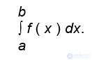
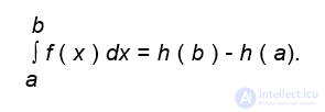
If the function f ( x ) is continuous at every point of the interval [ a, b ], then it has an antiderivative h ( x ) and its definite integral over the interval [ a, b ] equals the difference of the values of the function h at the points b and a:
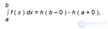
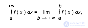
Improper integrals. In the case when the function f ( x ) or its antiderivative is not defined at the endpoints of the interval, the definite integral is computed by means of a limiting process:
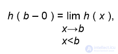
Improper integral:
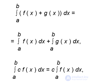
Properties of the definite integral
Definition of a complex number. A complex number is an expression of the form a + j b, where a, b – are real numbers, j – is a special symbol (the imaginary unit). The following notations are usually used:
a = Re ( a + j b )
( a – is the real part of the number a + j b ),
= Im ( a + j b )
( b – is the imaginary part of the number a + j b ); instead of a + j b one may write a + b j. Note that in mathematics the imaginary unit is denoted by the letter i, but in engineering this letter is used to denote electric current, so the symbol for the imaginary unit is the letter j. Real numbers are identified with complex numbers whose imaginary parts equal zero.
Representation of complex numbers by vectors. A complex number w is depicted by a vector (a directed segment) on a plane with a given coordinate system: the real part of w equals the projection of the directed segment onto the horizontal (real) axis, the imaginary part of w equals the projection of the directed segment onto the vertical (imaginary) axis.
The modulus of a complex number. The length | w | of the directed segment depicting a complex number is called the modulus of that complex number; by the Pythagorean theorem
| a + j b |2 = a2 + b2.
Algebraic operations on complex numbers. The vectors depicting complex numbers are added according to the parallelogram rule:
( a + j b ) + ( x + j y ) = ( a + x ) + j ( b + y )
(the real and imaginary parts of the terms are added separately). Complex numbers are multiplied like polynomials, with the square of the imaginary unit equal to -1:
( a + j b ) ( x + j y ) = a x + j b x + a j y + j b j y = ( a x - b y ) + j ( a y + b x );
Complex function of a real argument. A complex function of a real argument is a special case of a vector function, its components being two scalar functions.
The complex exponential function. The complex exponential function exp (( a + j b ) t ) assigns to each real number t a complex number
exp ( a t ) ( cos ( b t ) + j sin ( a + j b t )
Properties of the exponential function
exp ( u t ) exp ( v t ) = exp (( u + v ) t );
If Re ( u ) = 0, then
| exp ( u t ) | = 1;
if Re ( u ) < 0, then
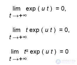
for any real number α; while if Re ( u ) > 0, then
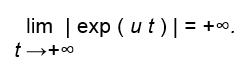
Differentiation of the complex exponential function:
( exp ( a + b j ) t )' = ( a + b j ) exp (( a + b j ) t ).
Polynomials. The function a0 x n + a1 x n-1 +…+ an-1 x + an is called a polynomial, and the complex or real numbers a0 ,… an - its coefficients; if a0 is nonzero, then the degree of the polynomial equals n. Polynomials of degree zero are constant functions; all coefficients of the zero polynomial equal zero.
Roots of a polynomial. The values of x at which a polynomial vanishes are called its roots. A polynomial of degree n > 0 has at least one root (complex or real); the total number of its roots does not exceed n.
Algebraic fractions. An algebraic fraction is a ratio of two polynomials.
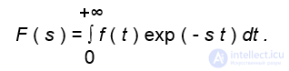
Definition of the Laplace transform. A complex function of a complex argument F ( s ) is called the Laplace transform of a real or complex function of a real argument f ( t ), defined on the interval ] 0, +∞ [, if for every s belonging to the domain of definition of the function F, the following equality holds
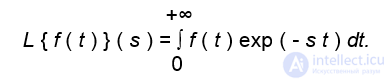
The Laplace transform of the function f ( t ) is often written in the form L { f ( t )}:
The inverse Laplace transform. The inverse Laplace transform L-1 { F ( s ) } ( t ) converts the function F ( s ) into the function f ( t ):
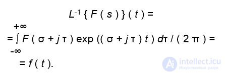
Strictly speaking, when computing the Laplace transform of the function f ( t ), we use the values of the function f for positive t. Therefore let us agree that f ( t ) = 0, when t ≤ 0. The inverse Laplace transform L-1 { F ( s ) } ( t ) is computed for positive values of the argument.
Properties of the Laplace transform. The direct and inverse Laplace transforms are linear:
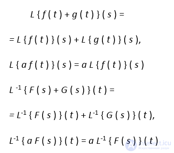
for any real or complex number a.
Table of correspondence between originals and images of functions. A function on which the operation of the Laplace transform is performed is called the original of the transform, and its result — its image (under the Laplace transform).
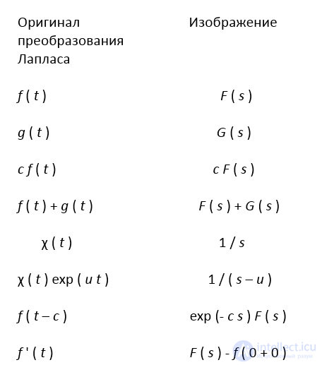

Comments