6. Methods of Spatial Propagation of Interference

The level of the wanted signal (or interference) at the receiver input, in the process of propagating from the source antenna to the receiving antenna, depends significantly on the radio wave propagation conditions. Calculation of the wanted signal and interference levels can be performed on the basis of rigorous methods used in radio wave propagation (RWP) theory, or, for specific selected propagation paths, using empirical formulas and engineering calculation methods in accordance with ITU recommendations.

Based on the mode of propagation, radio waves are divided into those propagating in free space (direct waves), ground waves, tropospheric waves, and ionospheric waves.

Freely propagating waves travel in a homogeneous or weakly inhomogeneous medium (in particular, in outer space) along rectilinear or near-rectilinear paths.

Ground radio waves propagate in close proximity to the Earth's surface and partially bend around the globe due to diffraction (diffracted waves).

Tropospheric radio waves propagate over considerable distances (up to about 1000 km) due to scattering in the troposphere and the guiding (waveguide) action of the troposphere.

Ionospheric or space waves propagate over large distances and can circle the globe as a result of multiple reflections from the ionosphere and the Earth's surface (> 10 m). This term also applies to waves that are scattered by ionospheric irregularities and reflected from ionized meteor trails (in the metre-wave range).

An important characteristic of radio wave propagation conditions is the value of propagation loss, showing how much the wave's power flux density is attenuated during propagation. When estimating propagation loss the entire path is usually divided into several regions or zones, and the possible mechanism of interference propagation for a given frequency range in each region is determined.

The line-of-sight region extends almost to the radio horizon (d 0,8^r₀ ) and, in the general case, is characterized by the presence of three types of waves: direct, reflected from the Earth's surface, and surface (ground) waves.

The diffraction or shadow region – the area of the Earth's surface where the direct wave is absent (d 1,2^r₀ ), and propagation occurs due to the wave bending around (diffraction from) the Earth's surface or terrain irregularities.

The penumbra region – intermediate between the line-of-sight and diffraction regions (0,8^r₀  d 1,2^r₀ ), where ^r₀ ̶ is the line-of-sight range.

The far tropospheric propagation region of radio waves (FTP) extends roughly from 100 to 1000 km. Waves in the 40…10000 MHz range can mainly propagate as tropospheric waves.

The ionospheric scatter region extends over a distance of 800 … 2400 km and covers the wave ranges 30 ... 100 MHz for scattering on ionospheric irregularities and 50...150 MHz for reflection from meteor trails.

Long-term and short-term propagation mechanisms are distinguished. It is generally accepted that RWP under line-of-sight conditions, as well as via tropospheric scatter or diffraction, constitute long-term mechanisms. They determine the propagation characteristics of both the wanted signal and interference. Short-term mechanisms include various anomalous tropospheric phenomena, such as temperature inversion with height, hydrometeor precipitation, the appearance of a tropospheric duct, and multipath, which, owing to their short duration, mainly determine only the spatial propagation characteristics of interference.

Table 6.1 – Data on RWP characteristics in various frequency bands

6.2 Characteristics of Wanted Radio Signal Propagation

Frequency range 10 kHz...30 MHz. At frequencies below 30 kHz, radio signal propagation losses approach the level of free-space propagation losses. In the VLF band, radio wave propagation in the waveguide mode between the ionosphere and the Earth's surface can be observed on a global scale.

In this frequency range it is important to take into account two different propagation modes: the ground-wave mode, which often determines the wanted signal levels, and the ionospheric-wave mode, by which interfering signals often propagate. The amplitude of the signal reflected from the ionosphere is characterized by pronounced diurnal fluctuations due to changes in the level of ionospheric absorption. The nature of ionospheric propagation implies that long-distance communication links will be subject to distortions caused by multipath, interference affecting the signal, and outages.

Frequency range 30 MHz ... 1 GHz. In this frequency range, except at the very lowest edge, the ionospheric radio-wave propagation mechanism does not operate. Weather effects are limited to superrefraction and duct propagation phenomena, which can be caused by inversions of the normal refractive-index gradient in the air. Other significant deviations from free-space propagation are tropospheric scatter and diffraction, caused by obstacles along the propagation path, including the curvature of the Earth's surface, as well as diffraction effects from terrain and buildings.

Frequency range 3...20 GHz. The radio-wave propagation factors described above (excluding ionospheric waves) also act in this frequency range. However, attenuation, scattering, and cross-polarization effects caused by hydrometeors must be taken into account. At frequencies above approximately 15 GHz, attenuation in atmospheric gases must also be considered.

Rain and other precipitation along the radio-wave propagation path can also create a number of problems. At frequencies above 10 GHz, attenuation due to raindrops can lead to significant degradation of signal quality.

During terrestrial radio-wave propagation under clear-sky conditions, fading can occur due to diffraction, multipath propagation in the atmosphere and along the Earth's surface, antenna defocusing, attenuation in atmospheric gases, and, in some regions, sand and dust storms.

Frequency range above 20 GHz. The main advantages of using this band, which provide extraordinary opportunities for frequency allocation and assignment, consist in the much larger available bandwidth and the small antenna sizes.

The main disadvantage here is the high susceptibility of propagation conditions to atmospheric phenomena, which cause large attenuation of radio waves and limit or preclude the use of many radio communication systems in this part of the radio spectrum. On the other hand, such effects can be exploited to provide protection against interference.

This frequency range is characterized by «windows», which are bands with relatively low attenuation, as well as absorption bands, where very high attenuation occurs. The transmission windows and absorption bands are determined primarily by the properties of atmospheric gases, mainly oxygen and water vapor. Absorption by oxygen is maximal at frequencies of 60 and 119 GHz, while absorption by water vapor is maximal in the frequency regions of 22 and 183 GHz.

Precipitation, especially in the form of rain, causes strong absorption and scattering of radio waves, as well as, to a lesser extent, rotation of the polarization plane of the radio waves. These effects can combine and contribute to significant attenuation. Calculations of specific attenuation at these frequencies depend to a large extent on the rain's microstructure (e.g., temperature, terminal velocity distribution, drop size and shape, etc.).

6.3 Characteristics of Interfering Radio Signal Propagation

Interfering signals (interference) between stations of different radio communication systems can arise not only from long-term but also from short-term propagation mechanisms. Interference propagation paths can have highly arbitrary characteristics. Therefore, the problem of reliably predicting interference levels is related to the difficulty of accounting for the wide variety of path types and parameters and their propagation conditions.

At certain periods of time, on a given section of the propagation path, a particular mechanism may predominate, or several interference propagation mechanisms may act simultaneously.

Line of sight. Interference levels can often increase significantly for short periods of time due to multipath propagation and focusing effects caused by the layered structure of the atmosphere.

Diffraction. Diffraction effects usually dominate beyond the line of sight and under normal conditions. Here, the curvature of the Earth and natural and artificial obstacles along the interference propagation path must be taken into account fairly accurately.

Tropospheric scatter. This mechanism determines the interference level for paths longer than 100...150 km, when the diffraction field becomes very weak. Nevertheless, in this case the interference will be at a fairly low level.

Surface duct. This is the most important short-term interference propagation mechanism and can cause high signal levels over large distances (more than 500 km over the sea). Under certain conditions, the level of such interference may exceed the level corresponding to free-space propagation.

Reflection and refraction from elevated layers. Reflection and/or refraction from layers at heights of up to several hundred meters is significant as a propagation mechanism, which, under favorable path geometry, produces interference levels higher than with diffraction propagation. In addition, the influence of this propagation mechanism can be significant at very long distances (up to 250...300 km).

Scattering by hydrometeors can be a potential source of interference produced by transmitters of terrestrial communication links and earth stations due to the effectively omnidirectional nature of radio-wave re-radiation.

Shielding effects from local irregularities (buildings, trees, etc.). This factor plays a protective role in interference propagation, since it reduces their reception levels to a certain extent.

6.4 Assessment of Radio Wave Propagation Loss

Free-space propagation. When radio waves propagate in free space, energy losses increase with distance due to the spherical spreading of the wave front, since, as distance increases, less energy falls on a unit area of the wave front. The power ^P_R at the output of the receiving antenna under such propagation conditions is determined by the expression

(6.1)

where A₀  20lg(4d /) – is the free-space propagation loss, P_T – is the power of the electromagnetic source delivered to the antenna; – wavelength, m; d – path length, m; G_T and G_R – the gains of the transmitting and receiving antennas, respectively.

Under real conditions, when propagating within line of sight, losses can increase not only with distance but also due to the influence of the Earth's surface itself and the absorption and scattering of electromagnetic energy in the ionosphere and troposphere.

In classical RWP theory, to account for losses, an attenuation factor F is introduced. Its value depends on a number of factors: the distance between the interference source and receptor, antenna mounting heights, wavelength, type of polarization, the terrain character of the propagation path, and the degree of atmospheric inhomogeneity. Taking the attenuation factor into account, formula (6.1) takes the form:

(6.2)

where A₀ = 32,5 +20lg( f )+ 20lg(d); dB; f – frequency; MHz, d – path length, km.

The conditions closest to free-space wave propagation are those of propagation on space communication links. In this case, the attenuation factor can be written as

A =A_t + A_i [dB], (6.3)

where: A_t – accounts for tropospheric losses due to wave absorption by oxygen, water vapor, and precipitation, A_i – accounts for the total losses caused by ionospheric absorption, scattering on ionized irregularities, and rotation of the wave polarization plane (Faraday effect).

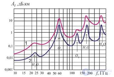
Figure 6.1 Frequency dependence of atmospheric attenuation:

1 at sea level, 2 4 km above sea level

Ground radio wave propagation under line-of-sight conditions. The line-of-sight region under normal refraction (characterized by an equivalent Earth radius a_eq equal to 4.3a , where a – the Earth's radius equal to 6371 km) extends to a distance d  r₀ (the line-of-sight distance or radio horizon) with a single antenna r_0[km]  4,12( h and with two antennas , where ^h_T and ^h_R – the heights of the transmitting and receiving antennas, respectively, measured in meters.

When calculating fields in the line-of-sight region, the conditions to be taken into account in RWP theory are classified according to the following criteria:

• antenna elevation height;
• distance from the transmitter (flat or spherical Earth)
• terrain relief (smooth, isolated pronounced obstacles, statistically rough surface).

Highly elevated antennas. If the heights of the receiving and transmitting antennas significantly exceed the wavelength ( 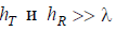) and the Earth's surface can be considered flat, smooth, and homogeneous, then the field at the receiving antenna location can be regarded as the result of interference between the direct wave and the wave reflected from the Earth's surface (Fig. 6.2).

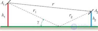
Figure 6.2 Propagation model under line-of-sight conditions

In the case of a perfectly conducting Earth surface, the attenuation factor can be determined using the formula

[dB], (6.4)

where 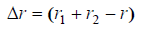– the path difference between the direct and reflected rays, the wavelength.

If the underlying surface cannot be considered perfectly conducting, then when calculating the attenuation factor, the complex reflection coefficient in the region significant for reflection must be taken into account, using the interference formula

[dB], (6.5)

where , the modulus and phase of the reflection coefficient over the section of the Earth's surface significant for reflection.

Statistically rough surface. To assess the degree of surface roughness in this case, the Rayleigh criterion is used, which the heights of the irregularities must satisfy: h_irr  / 8sin  , where is the grazing angle.

This is the condition under which a given surface can be considered smooth. If it is not satisfied, reflections acquire a diffuse character. The Rayleigh criterion does not take into account wave polarization, which, according to experimental data, has a significant effect on reflection. Surface roughness should be assessed not at a point but within the area bounded by the first Fresnel zone, and characterized by one scattering model or another.

When accounting for statistical surface irregularities, three waves are distinguished: direct, specularly reflected, and scattered. The overall field in the case of elevated antennas is determined using interference formulas for a smooth surface, but with a correction introduced into the reflection coefficient.

Most scattering models can be characterized, in simplified form, by two or three parameters (standard deviation and mean height of the irregularities, correlation interval). Surfaces with a Gaussian distribution of irregularity heights are the best studied. Surfaces of this type include, for example, the sea under moderate wave conditions.

Low-mounted antennas. Assuming that the Earth's surface is spherical, smooth, and homogeneous, and that the tropospheric refractive index decreases exponentially with height, in accordance with ITU-R recommendations, empirical formulas and graphs (a family of field-strength curves) are used to account for losses at frequencies from 10 kHz to 30 MHz E (dB(μV/m)). These curves (see Appendix 1) are plotted for a range of typical frequency values and underlying-surface characteristics (relative permittivity and conductivity) under the following assumptions:

• the transmitting and receiving antennas are located at ground level;
• the radiating element is a short vertical monopole.

Assuming that such a vertical antenna is located on the surface of a perfectly conducting flat Earth and radiates a power of 1 kW, the field strength at a distance of 1 km will be 300 mV/m; this corresponds to an effective radiated moment of 300 V:

• the curves are plotted for distances measured along the curved surface of the Earth;
• the curves give the values of the vertical component of the radiated field strength, i.e., the component that can be effectively measured in the far field of the antenna.

The total propagation loss can be determined from the following equation

(where f in MHz)

, [dB].

This data, with an error of less than 1 dB, corresponds to the field at a distance r , if kr 10, where k = 2π/λ. At closer distances, the influence of the near field (i.e., the induction field and the static field) can be taken into account by adding to the field strength (in dB) the value

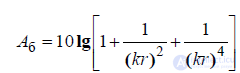[dB].

The curves given in figures similar to Fig. 6.3 can be used to determine radio-wave propagation parameters also for mixed paths (inhomogeneous smooth Earth surface), as follows. Such paths may, for example, be formed from three sections ^S₁, ^S₂, S₃ of length ^d₁, ^d₂, d₃ , with parameters 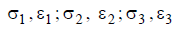, as shown below:

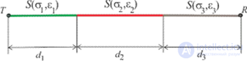
Figure 6.3 Mixed propagation path

The Millington method, used to determine radio-wave propagation parameters on mixed paths, is the most accurate of all available methods and satisfies the reciprocity condition.

This method assumes that for the path sections S₁, S₂, S₃, each of which is individually considered homogeneous, propagation curves exist for the various terrain types corresponding to these sections, all of which are obtained for the same radiation source (T), and can be recalculated for any other radiation source.

For a given frequency, the curve corresponding to section S₁ is selected, and then the field E₁(d₁) in dB(μV/m) at a distance d₁ is determined. After that, the curve corresponding to section S₂ is used to determine the fields E₂(d₁) and E₂(d₁ +d₂) and, similarly, using the curve for section S₃ the fields E₃(d₁ +d2) and E₃(d₁ +d₂ +d₃) etc.

The field strength of the received signal, E_R, is then determined as:

E_R = E₃(d₃) -E₂(d₃) +E₂(d₃ +d₂) -E₃(d₁ +d2) + E₃(d₁ +d₂ +d₃) . (6.6)

The reverse procedure is then carried out, and, denoting by the index T the transmitter, and by the index R the receiver, we obtain the expression for the field strength

E_T =E₁(d₁) - E₂(d₁) + E₂(d₁ +d₂) -E₁(d₃ +d2) + E₁(d₁ +d₂ +d₃).

The required field-strength value is determined as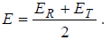

The Millington method is generally simple to use and can be applied to a larger number of sections, especially when computer programs are used for the calculations.

Methods for predicting interference level in the range 0.7…100 GHz are contained in ITU-R Recommendation P.452.

The basic propagation loss , dB, not exceeded for p (%) of the time can be calculated using the formula:

_g [dB],

where the parameter A_g accounts for the total absorption by atmospheric gases, and E_s(p) is a correction parameter accounting for multipath and focusing effects

[dB].

Propagation of interfering signals (IS) due to diffraction. The basic transmission loss, not exceeded for p % of the time

[dB],

where

A_d (50%) — diffraction loss for p = 50%;

diffraction loss for β₀ %;

F_i(p); — interpolation parameter.

Propagation of interference via tropospheric scatter. For small percentages of time, it is difficult to establish the actual tropospheric propagation effect, since there are also secondary effects of this propagation mode, such as tropospheric ducting and layer reflections. This allows a continuous prediction of the basic transmission loss within the time percentage range 0.001% <p < 50%.

The basic transmission loss A_s dB, not exceeded for p < 50%, can be determined using the formula:

[dB],

where – the scattering angle along the propagation path, mrad; L_f frequency-dependent losses,

gain loss along the path, G_T and G_R the gains of the transmitting and receiving antennas, respectively; A_g gas absorption.

Waveguide (ducting) propagation of interference and propagation via layer reflections. The basic transmission loss A_w for this interference propagation mechanism is determined by the formula

[dB],

where A_f the total constant loss (excluding losses due to local terrain/infrastructure irregularities), caused by the anomalous propagation structure within the atmosphere, A_d (p) the loss due to anomalous propagation conditions, depending on the scattering angle.

Shielding of interference by local irregularities. This interference propagation mechanism is the source of additional diffraction losses when antennas are placed amid local terrain/infrastructure irregularities (buildings, vegetation, etc.). Losses of this kind are calculated for the nominal parameters of typical irregularities (their heights and distances from the antenna), given in Table 6.2.

Table 6.2 – Parameters of typical irregularities

When reliable information on such irregularities is unavailable, losses due to scattering by infrastructure irregularities should not be taken into account.

Additional loss due to shielding by local irregularities

[dB],

where d_k the distance from the location of the irregularity to the antenna, km; h – the height

of the antenna above the local ground level, m; h_a the nominal height of the irregularity above the local ground level, m.

Propagation of interference due to scattering by hydrometeors. The model of this propagation mechanism is based on the following assumptions:

- scattering occurs only within a cylindrical rain cell, whose diameter depends on the rain intensity in the cell. Within the rain cell, the rain intensity is constant up to the rain height. Above the rain height, a linear decrease in reflectivity is assumed; - attenuation occurs both inside and outside the cell, but only below the rain height.

This model can be used to calculate interference levels both on long paths (more than 100 km) and short ones (down to a few kilometers), with arbitrary elevation angles at both terminals, as well as on paths with lateral scattering (i.e., outside the great-circle plane) and on interference propagation paths through the side lobe of one station's antenna radiation pattern and the main lobe of the other station's antenna radiation pattern.

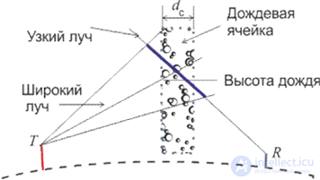
Figure 6.4 - Propagation path geometry

The diameter of the rain cell d_c km, depends on the rain intensity R, mm/h, as d_c 3,3R^0,08 . The cell is centered at the point of intersection of the antenna radiation patterns of the interacting

stations, as shown in Fig. 6.4

The transmission loss (dB) due to scattering by hydrometeors for a given rain intensity R and rain height h_R can be expressed by the relation

,

where _E is the antenna efficiency parameter (_E <1), a typical value _E  0,6 ; d_T the distance between stations through the scattering volume (SV), km; f frequency, GHz; z_R the reflectivity parameter of a unit rain volume below or above the rain height, mm⁶/m³, z_R  400R(p)^1,4 ; R( p) the one-minute mean rain intensity at the point, exceeded for

the p % of the time;S — a correction parameter for the deviation of the scattering law from Rayleigh at frequencies above 10 GHz; C the effective scattering transfer function.

6.5 Accounting for Loss in Urban Environments

When designing communication systems for mobile objects in urban environments, in order to solve many problems it is necessary to be able to calculate the characteristics of both the wanted signal and interference at any point in space within the entire service area.

The urban environment has specific radio-wave propagation conditions, such as shadow zones, multiple reflections, and wave scattering, which produce fields with a complex interference structure and sharp spatial variations in wanted-signal and interference levels.

The multipath nature of radio-wave propagation, in which waves arrive at the reception point from different directions and with different time delays, gives rise, in particular, to intersymbol interference phenomena.

When developing communication systems for mobile objects in an urban environment, the following models are currently used to calculate propagation loss.

1. The Okumura model (Okumura). Graphs allowing determination of the median signal value, and to some extent accounting for the particular features of a given city or individual urban districts, were obtained by Okumura. The Okumura model is one of the most widely used models for predicting signal levels in urban environments.

This model is applicable in the frequency range from 150 to 1900 MHz (often extrapolated to 3000 MHz) for distances from 1 to 100 km, with transmitting antenna heights from 30 to 1000 m. It formally proposes using the following equation for loss calculation, in which all quantities are given in decibels

(6.7)

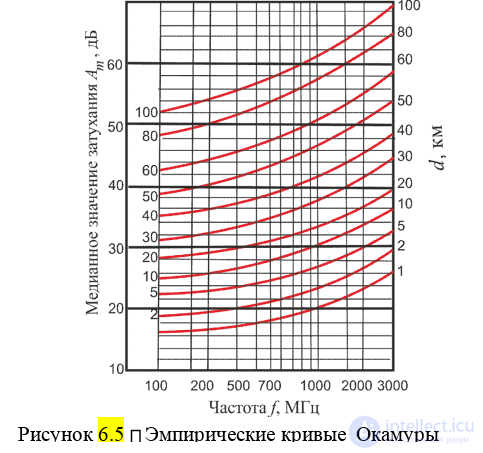
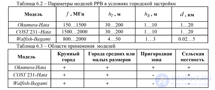
where A₀ – the free-space propagation loss; A_m – the median attenuation value in urban conditions, at an effective height (the height of the antenna's electrical center above the averaged surface level along the propagation path) of the transmitting antenna h_T = 200 m and a receiving antenna height h_R = 3 m; G(h_T ) – the coefficient accounting for the transmitting antenna height; G(h_R ) – the coefficient accounting for the receiving antenna height; K – a correction coefficient accounting for the surroundings, water surface, isolated obstacle, etc. The attenuation values A_m , which depend on the distance d and frequency f , can be found from the curves shown in Fig. 6.6. Parameter values for this and the models described below are given in Tables 6.2 and 6.3.

1. The Okumura–Hata model (OkumuraHata). The essence of this model consists in approximating Okumura's graphs with specially selected formulas for various territory zones, conventionally divided into large city, medium and small city, suburban, rural, and open areas.

(6.8)

The drawbacks of this model are the same as those of the original Okumura model, and lead to an underestimation of losses for frequencies above 1.5 GHz.

1. The modified Hata model (COST 231Hata). The advent of communication systems operating in the frequency range around 2 GHz spurred further research within the COST project (Cooperation for Scientific and Technical Research), leading to the extension of the Okumura–Hata model to the frequency range from 1.5 to 2 GHz. This modification, called COST 231, is valid for antenna height values h_T of 30...200 m and h_R of 1...10 m, and distances between them d of 1...20 km. This model cannot be used at d less than 1 km, or when estimating signal levels in street conditions with tall buildings.

where D – a constant; for a suburban area D= 0 dB, and for urban development D = 3 dB.

For small and medium-sized cities, the correction factor

for large cities:

1. The Walfisch-Ikegami model (COST 231 Walfish-Ikegami ). This model can be applied in cases where the transmitting antenna (e.g., a base station antenna) is located either above or below the rooftop level of urban buildings.

Two situations are considered: in one case the transmitting and receiving antennas are in line-of-sight conditions, and in the second – outside line of sight.

In the «line-of-sight» situation, the signal attenuation A_0 is calculated using a formula that includes only two parameters: the distance d (km) and the frequency f (MHz)

(6.9)

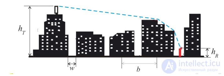
When calculating attenuation in the «non-line-of-sight» situation, the set of empirical factors accounted for by the calculation formula includes the heights of the base-station antenna ^h_T and the mobile-station antenna ^h_R the street width w, the distance b between buildings, building height, and the orientation of streets relative to the signal propagation direction.

In general terms, the formula describing the loss in this case consists of three terms – the free-space propagation loss A₀  32,5 20lg( f )  20lg(d); the loss

A_rts (rooftop-to-street) due to diffraction and scattering of waves caused by multiple diffraction from rows of buildings. This type of loss was accounted for in the Ikegami model, which was used within the COST 231 project. In addition, the model under consideration accounts for the loss A_msd (multiple screen diffraction) due to diffraction of waves over building rooftops, by which the signal reaches the moving object, as well as due to multiple diffraction from rows of buildings

6.6 Radio Wave Propagation Inside Buildings and Premises

Considerable attention has recently been paid to the problem of radio-wave propagation inside buildings and premises. This is mainly due to the creation of local networks and the need to form a reliable information environment for the staff of enterprises and institutions. The presence, inside a building, of walls, partitions, furniture, radio-electronic equipment, people, and other objects creates a complex environment for the propagation of wanted signals and interference. Conditions for radio-wave propagation inside premises differ substantially from those for propagation in free space.

The main effects observed under these conditions are multipath propagation, caused by multiple reflections from walls and other objects, diffraction from the numerous sharp edges of objects located inside the room, and radio-wave scattering. These effects create a complex interference structure of the electromagnetic field, which changes greatly as people and other objects move around.

Description of EMC conditions inside buildings. Most models used for calculations inside buildings are based on the formula describing radio-wave propagation in free space. However, the presence of walls, floors, furniture, people, and other objects has a significant influence on the nature of radio-wave propagation. The diversity of conditions makes it necessary to use empirical models based on numerous experiments investigating radio-wave propagation conditions inside premises.

Models for describing the characteristics of radio-wave propagation inside buildings differ from traditional channel models, since the coverage area is significantly smaller than in urban conditions, and the radio-wave propagation conditions are more varied. Radio-wave propagation inside buildings is determined by the building type, layout, and the properties of the construction materials used.

The levels of both the wanted signal and interference depend on whether the doors in rooms are open or closed, and on antenna placement (at table level or near the ceiling). Inside buildings there are numerous walls and partitions, and various objects, which can significantly affect the formation of the electromagnetic field structure inside and outside the building. Walls and partitions inside buildings are usually made of construction materials with different electrical properties; mainly there are two types of walls: «hard» walls, which are part of the building's structure, and «soft» walls – partitions, which, in particular, can be movable.

Attenuation during propagation between different floors is determined not only by the external dimensions and material of the building, but also by the construction of the floor slabs, the external surroundings, the number of windows in the building, and the character of the wall surfaces. The loss in decibels inside buildings A_sf is determined by the expression

(6.10)

where r₀ – the distance between the receiving and transmitting antennas in space; r – the distance along the radio-wave propagation path; n 1.6...3.3 – a coefficient depending on the building type and surrounding structures; X_ – a random variable following a normal distribution with a variance of 3.0...14.1. This model gives a loss value that differs from the experimentally measured value by no more than 4 dB.

One of the many empirical models describes the total loss A_mf for the case of radio-wave propagation between floors using the formula

, (6.11)

where n_SF 2.8 – a coefficient characterizing propagation within a single floor

(self floor); K_e – a coefficient characterizing attenuation between floors (12.9…16.2 dB – for propagation through one floor; 18.7…27.5 dB – through two floors, and 24.4…31.6 dB – through three floors).

In many cases, when studying radio-wave propagation in urban environments or inside buildings and premises, it becomes necessary to calculate the wave transmission coefficient through walls, partitions, and other layered media. Some information on the characteristics of wall materials is given in Table 6.4.

Table 6.4 – Electrical characteristics of construction materials