4. Models of the spectrum envelope and radiation parameters of a radio transmitter

4.1 Fundamental emission

In practice, the emissions of radio transmitters, as a rule, occupy a wider frequency band than necessary. The bandwidth of the fundamental emission is determined from the values of the boundary frequencies of the band outside of which the power of the spectral components of the signal does not exceed a specified relative level. The reference level depends on the type of modulation of the useful signal.

In the most common cases, the zero level is set at the carrier amplitude in the absence of modulation, while for pulse signals the maximum value of the spectrum envelope is taken as the zero level.

The use of several measurement levels makes it possible to monitor out-of-band emissions. To measure the width of the occupied frequency band from the values of the boundary frequencies at a specified emission level (in decibels), it is convenient to use conventional spectrum analyzers.

The existence of standards for out-of-band emissions makes it possible to construct the power spectrum envelope for any emission class.

Information on the power spectrum envelope is used at the stage of EMC analysis of radio equipment. Usually the exact shape of the envelope is not of significant importance, and this allows functional dependences of various kinds to be used to approximate the envelope.

For practical purposes, the simplest approximation of the power spectrum envelope by straight-line segments is most often used

(4.1)

where – value of the envelope at a detuning relative to the center of the spectrum by the amount

– number of the approximated section of the envelope; ^f_i – width of the approximated section; A_i - rate of change of the envelope on the i -th approximation section, dB/dec.

The slope of the limiting line ^A_i characterizes the rate of decrease of the power of the spectral components of the emission power.

The functional dependence (4.1) makes it fairly convenient to use a logarithmic scale on the frequency axis when graphically constructing the spectrum envelope.

Figure 4.1 shows the limiting curve of the emission power spectrum.

With a large number of radio equipment units, for a quick EMC assessment it is more convenient to use an approximation of the form (4.1) not for the emission class, but for the type of modulation. The coefficient values for the corresponding models are given in Appendix 2 (Table A2.1).

The maximum attenuation of the spectral components is assumed to be –100 dB.

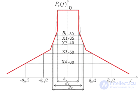
Figure 4.1 – Limiting curve of the emission spectrum of class A3E:

B_c – width of the control frequency band; B_Xi – bandwidth at level X_i

4.2 Out-of-band emission

The out-of-band emission spectrum is the part of the power density spectrum or the power spectrum (in the case of a discrete spectrum) that lies outside the necessary frequency band. An insignificant, and therefore disregarded, part of the out-of-band emissions may also lie in the region of spurious emissions.

The spectrum of the fundamental emission is determined by the type of modulation. The part of the spectral power of the useful signal that lies outside the necessary frequency band forms the out-of-band emission. Thus, the out-of-band emission shown in Fig. 3.1 is created by spectral components at . Signal out-of-band emissions can occur due to a non-optimal choice of the modulating signal shape, the nonlinear nature of the transmitter's modulation characteristic or of the modulating signal shaping path, and overmodulation effects.

The permissible out-of-band emission level is determined by the total value of the average power radiated at frequencies lying outside the necessary frequency band. This level is standardized as a percentage of the average emission power and should be minimal so as not to create radio interference in adjacent radio channels.

4.3 Harmonic and subharmonic emissions

After the fundamental emission of the transmitter, harmonic emissions have the most significant level.

There are two causes of the occurrence of emissions at harmonics:

• in transmitters of the meter band and longer-wave bands, these are power amplifier stages operating with current cutoff angles of less than 180^o;
• in higher-frequency transmitters (decimeter and shorter waves) they are formed in the output electrovacuum devices.

For example, in magnetrons the level of the second harmonic reaches values

(-30...-40) dB, in TWTs (-20...-30) dB, and in broadband TWTs (-7...-10) dB.

Attenuation of harmonic emissions is achieved by circuit means (push-pull circuits, negative feedback, etc.), as well as by filtering. However, complete suppression of these emissions cannot be achieved.

The levels of these emissions depend on many random factors that cannot always be taken into account. In EMC analysis, the power level of a spurious emission (expressed in decibels: dB/mW) is usually treated as a random variable with a normal distribution law. In this case it is fully characterized by the first two moments of the distribution law: the mean value and the variance.

The frequency dependence of the mean power value P_g in dBW at the frequency of the n -th harmonic f_n is commonly described by a simplified expression of the form

(4.2)

where P_T ( f_0T ) – mean power level of the fundamental emission at the transmitter's operating frequency f_0T ; A_g and Q_g – constant coefficients.

The quantity A_g – characterizes the decay rate of the spurious emission level as a function of its detuning relative to the frequency of the fundamental emission, and Q_g – is the attenuation relative to the fundamental emission. These coefficients are usually determined on the basis of statistical processing of measurement results

Note that the model described by expression (4.2) is of a general nature and can be used to describe not only harmonic emissions, but also other types of spurious emissions. In this case, the model coefficients differ for different types of spurious emission.

Having sample values of the emission power P_T ( f_i ) at the frequencies f_i , corresponding to the harmonics, it is also possible to calculate the second moment of the distribution the variance

In cases where information on the parameters of model (4.2) is unavailable, it is possible to use the data given in Appendix 2 (see Table A2.2).

4.4 Combination, intermodulation, parasitic, and noise emissions

Recall that combination emission arises as a result of interactions in radio transmitters between oscillations at the carrier frequency and oscillations forming the carrier frequency, as well as their harmonics.

Spurious combination emissions are characteristic of transmitters containing band exciters. They are formed in the exciter or frequency synthesizer of the transmitter, when the operating frequency is formed from one or more frequencies of the self-oscillator or the reference crystal oscillator.

In the synthesizer, the grid of operating frequencies is created by nonlinear transformations of several oscillations with frequencies f₁ , f₂ , f₃ … , usually in a decade ratio f₂ =10 f₁ , f₃ =10 f₂ … .

As a result of their mixing, components appear at frequencies , where p, q, m – are positive integers. All of them, together with the useful

oscillation of the operating carrier frequency, are present at the synthesizer output.

Using filters, the required frequency is extracted. If the initial frequencies are chosen incorrectly, or filtering is poor, oscillations of undesirable frequency combinations can penetrate to the transmitter output.

Thus, for example, if certain frequencies satisfy the inequality

where f_f – is the tuning frequency of the mixer filter, B_f – is the passband of this filter, then a significant level of combination emission will be observed in the emission spectrum of the transmitter being formed.

The formation of the frequency grid by the analysis method is characterized by the fact that the exciter's operating frequency is created by a generator with smooth frequency tuning and is stabilized using one or another automatic frequency control method. Compared with the synthesis method, the analysis method provides a lower level of combination frequencies.

Model (5.2) is used for the analytical description of combination emission levels. The structure of the power spectrum of the combination emission is determined by the structure of the spectrum of the master oscillator and the nature of the nonlinear transformations.

Intermodulation emission arises when transmitters of different purposes operate on closely spaced antennas or on a single broadband antenna. This emission is especially important to take into account in EMC analysis at sites with a large number of transmitters and a small area for the placement of radio equipment (mainly at mobile sites). Intermodulation emissions are formed according to the same laws as combination emissions. However, not all intermodulation emissions present the same degree of danger. This danger is determined both by the power of this emission and by the magnitude of the detuning of the intermodulation oscillation frequency relative to the tuning frequency of the receiver.

When two transmitters with operating carrier frequencies f₁ and f₂ interact, intermodulation components arise at frequencies , where m,n are integers. There is currently no general analytical formula for calculating the power of intermodulation emission. Values of some intermodulation frequencies are given in Table 4.3.

Table 4.3 – Intermodulation frequencies

The total number of intermodulation frequencies increases with increasing intermodulation order 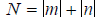. The magnitude of the detuning of even-order intermodulation frequencies relative to the transmitter's operating frequency is large, and therefore their levels are strongly attenuated.

The most dangerous are odd-order intermodulation emissions, and primarily those located closer to the transmitter's carrier frequency. Third-order intermodulation frequencies are the closest in frequency to the transmitter's fundamental emission frequency. They can fall within the passband of the output stage, are little attenuated by the transmitter's selective circuits, and therefore have the greatest interfering effect.

Fifth- and seventh-order intermodulation components can also lie within the amplification band of the output stages, but their power is significantly lower than that of third-order components.

The level of odd-order intermodulation products can be described by means of an empirical formula

P_I = C_I + kP_i ,

where P_I – is the power of the intermodulation interference, dB/mW; P_i – is the power of the interfering transmitter; C_I – is the intermodulation constant; k – is the proportionality coefficient, dB/mW.

To reduce the level of intermodulation emissions, filtering is applied, and coupling between antennas is also reduced by their rational placement and the use of spatial decoupling structures.

The parameters ^C_I and k, based on the results of measurements of the interference power and the intermodulation emission power at a given detuning, can be calculated using the following formulas:

where indices 1 and 2 denote the measurement number.

Noise emission is caused by the intrinsic noise of the transmitter's elements and by parasitic modulation of the carrier as a result of noise processes. Noise emissions are characterized by the power spectral density (absolute or relative to the level of the fundamental emission) and by the width of the occupied frequency band. The intensity of a transmitter's noise emission depends on the circuit design, its purpose, the frequency range, the element base used, and the detuning Δf relative to the frequency ^f_0T of the fundamental emission. To quantitatively describe noise emissions, an expression analogous to (4.2) can be applied

(4.3)

where P_N (Δf ) – is the power level (dBW) of the noise emission at a detuning Δf from the frequency of the fundamental emission; A_N – is the decay rate of the noise emission (dB/dec); Q_N – is the attenuation of the noise emission power in the occupied frequency band B_o relative to the fundamental emission.

For broadband and narrowband radio transmitters, the coefficient A_N is equal to –3 and –15 dB/dec, respectively, while Q_N =-60...-80 dB.