
Lecture
Это окончание невероятной информации про радиопеленгация.
...
] : 206 Even with special processes used to reduce lead length, [ 23 ] such as frame-grid construction, as in the EF50 , and planar construction, [ 20 ] : 192 very few tubes could operate above UHF .In the 1930s, intensive research was carried out to develop transmitting tubes specifically designed for the microwave range, which included, in particular, the klystron [ 24 ] [ 20 ] : 201 , cavity magnetron [ 20 ] : 347 [ 24 ] : 45 and the traveling-wave tube (TWT). [ 20 ] : 241 [ 24 ] : 48 After the successful development of these tubes, large-scale production began in the following decade.
Microwave signals have short wavelengths, which leads to a significant improvement in target resolution compared to radio-frequency systems. This allows for better identification of multiple targets and also provides improved direction-finding accuracy. [ 25 ] In addition, the antennas are small, so they can be assembled into compact arrays, and moreover they can produce well-defined radiation patterns that provide narrow, high-gain beams, which are preferred for radars and data links .
Other advantages of the new microwave range included the absence of fading (often a problem in the shortwave radio band ), and a significant increase in signal bandwidth compared to the already congested radio-frequency bands in use. In addition to being able to receive far more signals, it became possible to use spread-spectrum and frequency-hopping techniques .
Once microwave technology became widespread, it was rapidly adopted by both military and commercial users of this frequency range.
Antennas for direction finding must meet different requirements than antennas for radar or communication links, where a narrow-beam, high-gain antenna is usually an advantage. However, when performing direction finding, the bearing of the source may be unknown, so antennas with a wide radiation pattern are usually chosen , even though they have a lower gain along the antenna boresight axis . In addition, the antennas are required to cover a wide range of frequencies.
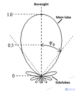
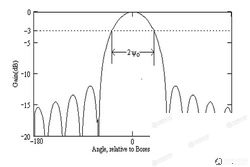
The figure shows the normalized polar diagram of a typical antenna gain pattern in the horizontal plane. The half-power beamwidth of the main lobe is 2 × Ψ 0. It is preferable, when using amplitude-comparison methods for direction finding, for the main lobe to be approximated by a Gaussian characteristic. Although the figure also shows the presence of side lobes , they do not present a serious problem when the antennas are used in a direction-finding antenna array.
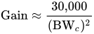
As a general rule, antenna boresight gain is related to beamwidth. [ 26 ] : 257 For a rectangular horn,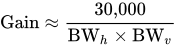 where BW h and BW v — are the horizontal and vertical antenna beamwidths, respectively, in degrees. For a circular aperture with beamwidth BW c this is
Two types of antennas are widely used for direction finding: spiral antennas with a cavity at the back, and horn antennas .
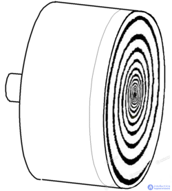
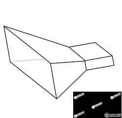
Spiral antennas are capable of providing very wide bandwidth and have a nominal half-power beamwidth of about 70 degrees, which makes them very suitable for antenna arrays containing 4, 5, or 6 antennas. [ 18 ] : 41
For larger arrays requiring a narrower beamwidth , horns can be used. The bandwidth of horn antennas can be increased by using dual-ridge waveguide feeds and by using horns with internal ridges.
Early microwave receivers were typically simple «crystal video receivers» , which used a crystal detector followed by a video amplifier with a compressive characteristic to extend the dynamic range. Such a receiver was wideband but not very sensitive. However, this lack of sensitivity could be tolerated because of the «range advantage» enjoyed by the DF receiver (see below).
The klystron and TWT are linear devices and, in principle, could be used as receiver preamplifiers. However, the klystron was completely unsuitable, since it is a narrowband and extremely noisy device , while the TWT, although potentially more suitable, has poor matching characteristics and large dimensions, which makes it unsuitable for multichannel systems using a preamplifier for each antenna. Nevertheless, a system has been demonstrated in which a single TWT preamplifier selectively picks signals from the antenna array. [ 33 ]
Transistors suitable for operation at microwave frequencies appeared in the late 1950s. The first of these was the metal-oxide-semiconductor field-effect transistor (MOSFET). It was followed by others, such as the metal-semiconductor field-effect transistor and the high electron mobility transistor (HEMT). Initially, discrete transistors were built into stripline or microstrip circuits, but then microwave integrated circuits appeared. Thanks to these new devices, it became possible to create low-noise receiver preamplifiers, which significantly increased sensitivity and, consequently, the detection range of radio direction-finding systems.
The DF receiver has a detection-range advantage [ 35 ] compared to a radar receiver. This is because the signal power at the DF receiver, due to the radar transmission, is proportional to 1/ R² , whereas the signal power at the radar receiver from the reflected signal is proportional to σ / R⁴ , where R — is the range, and σ — is the radar cross section of the DF system. [ 36 ] This means , that the signal power at the radar receiver is significantly lower than at the DF receiver. Consequently, despite its low sensitivity, a simple crystal-video DF receiver is usually able to detect a radar's signal transmission at a greater range than that at which the radar's own receiver is able to detect the presence of the DF system. [ 18 ] : 8
In practice, the advantage is reduced by the ratio of antenna gains (typically 36 dB and 10 dB for the radar and ESM, respectively), and by the radar's use of spread-spectrum techniques, such as chirp pulse compression , to increase its receiver's processing gain. On the other hand, the DF system can partially offset this advantage by using sensitive low-noise receivers and applying «stealth» techniques to reduce its own radar signature [ 29 ] : 292, as in the case of stealth aircraft and stealth ships .
The move to microwave frequencies meant a re-evaluation of the requirements for the direction-finding system. [ 37 ] The receiver could no longer rely on a continuous stream of signals to make measurements. Radars with their narrow beams would illuminate the direction-finding system's antennas only intermittently. Furthermore, some radars seeking to avoid detection (for example, radars used by smugglers, hostile ships, and missiles) would radiate their signals infrequently and often at low power. [ 38 ] Such a system is called a low probability of intercept (LPI) radar . [ 39 ] [ 40 ] In other applications, such as microwave data links, the transmitter antenna may never actually be pointed at the direction-finding receiver at all, so reception is possible only through signal leakage from the side lobes of the antenna. In addition, covert data links [ 41 ] may transmit a high-data-rate burst only very rarely.
In general, to meet modern conditions, a wideband microwave DF system must have high sensitivity and 360-degree coverage in order to be able to detect single pulses (often called amplitude monopulses ) and to achieve a high «probability of intercept» (PoI). [ 42 ]
Amplitude comparison has become a popular method of direction finding, since such systems are relatively simple to implement, have good sensitivity, and, importantly, a high probability of signal detection. [ 43 ] : 97 [ 18 ] : 207 An array of four or more directional antennas, arranged at an angle to each other, is typically used to provide 360-degree coverage. [ 44 ] : 155 [ 18 ] : 101 [ 45 ] : 5–8,7 [ 43 ] : 97 [ 46 ] Direction finding using phase-comparison methods can provide better bearing accuracy, [ 45 ] : 5–8,9 but the processing is more complex. Systems using a single rotating parabolic antenna are more sensitive, small, and relatively simple to implement, but have a poor probability of intercept. [ 42 ]
Typically, to determine the direction of the incoming wavefront, the signal amplitudes in two adjacent channels of the antenna array are compared, but sometimes three adjacent channels are used to improve accuracy. Although the gains of the antennas and their amplifier chains must be precisely matched, careful design and manufacture, together with effective calibration procedures, can compensate for equipment shortcomings. The overall direction-finding accuracy is from 2° to 10° (rms) [ 45 ] [ 47 ] when using this method.
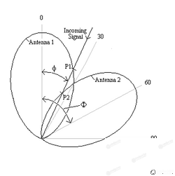
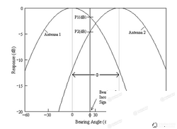
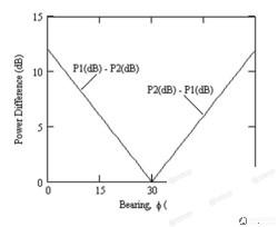
Two-channel direction finding, using two adjacent antennas of a circular array, is achieved by comparing the power of the strongest signal with the power of the second-strongest signal. The direction of the incoming signal within the arc subtended by two antennas with an included angle of Φ , can be determined by comparing the relative powers of the received signals. When the signal is along the boresight of one of the antennas, the signal at the other antenna will be about 12 dB lower. When the signal direction is midway between the two antennas, the signal levels will be equal and about 3 dB lower than the boresight value. At other bearing angles φ some intermediate ratio of signal levels will determine the direction.
If the antenna's main lobe pattern has a Gaussian characteristic, and the signal power is expressed logarithmically (for example, in decibels (dB) relative to the boresight value), then there is a linear relationship between the bearing angle φ and the power-level difference, i.e.: where P1 ( dB) and P2 (dB) — are the output signals of the two adjacent channels. The sketch shows a typical plot.
To provide circular coverage (360°), the antennas of the circular array are selected in pairs according to the signal levels received by each antenna. If the array has N antennas arranged with an angular spacing (included angle) of Φ, then Φ = 2π/ N radians ( = 360/ N degrees).
If the main lobes of the antennas have a Gaussian characteristic, then the output P 1 ( φ ) as a function of the bearing angle φ is given by the formula [ 18 ] : 238
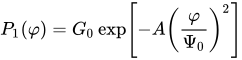
where
A second antenna, pointed at an angle Φ and having the same gain G0 , produces an output signal.
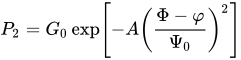
Comparing the signal levels,
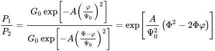
The natural logarithm of the ratio equals

Rearranging: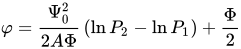
This demonstrates a linear relationship between the difference in output signal levels, expressed on a logarithmic scale, and the bearing angle φ .
Natural logarithms can be converted to decibels (dB) (where dB denotes the gain relative to the boresight axis) using the following formula: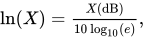 Thus, the equation can be written.

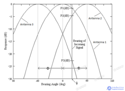
Improved bearing accuracy can be achieved if amplitude data from a third antenna are included in the bearing computation. [ 48 ] [ 44 ] : 157
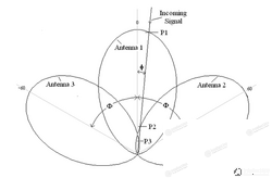
For a three-channel direction-finding (DF) system with three antennas spaced at an angle of Φ, the direction of the incoming signal is determined by comparing the signal power of the channel with the largest signal to the signal powers of the two neighboring channels on either side of it.
For antennas arranged in a circle, three antennas are selected based on the level of the received signal, with the largest signal falling on the center channel.
When the signal is along the boresight axis of antenna 1 ( φ = 0 ), the signals from the other two antennas will be equal and about 12 dB lower. When the signal direction is midway between two antennas ( φ = 30° ), their signal levels will be equal and about 3 dB below the boresight-axis value, while the third signal will be about 24 dB lower. At other bearing angles φ the direction will be determined by some intermediate ratio of signal levels.
For a signal arriving from a direction φ, taken here as the direction to the right of the boresight axis of antenna 1, the output signals of the three channels will be as follows:
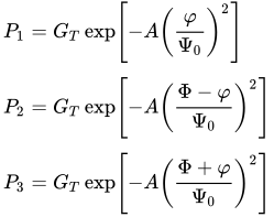
where G T — the total gain of each channel, including the boresight-axis gain, and is assumed to be the same for all three channels. As before, in these equations the angles are expressed in radians, Φ = 360/ N degrees = 2π/ N radians and A = – ln(0.5) .
As before, these can be expanded and combined to give:
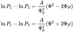
Eliminating
 and rearranging:

where:
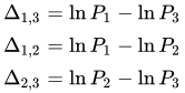
Here the difference values are given in nepers, but can also be expressed in decibels .
The bearing value obtained from this equation does not depend on the antenna beamwidth ( = 2Ψ 0 ), so this value does not need to be known to obtain accurate bearing measurements. In addition, there is a smoothing effect on bearing values near the axis of the middle antenna, so there is no discontinuity in bearing values in this region when the incoming signal moves from left to right (or vice versa) across the axis, as can happen with two-channel processing.
Many sources of bearing error, such as mechanical defects in the antenna structure, poor matching of receiver gains, or non-ideal antenna radiation patterns, can be compensated for by calibration procedures and correction lookup tables, but thermal noise will always be a factor degrading accuracy. Since all systems generate thermal noise [ 49 ] [ 50 ], at a low incoming signal level the signal-to-noise ratio in the receiver channels will be low, and the accuracy of the bearing estimate will suffer.
In general, guidance on bearing uncertainty is given in [ 45 ] [ 51 ] : 82 [ 31 ] : 91 [ 52 ] : 244

for the signal at the crossover point, but where SNR 0 — is the signal-to-noise ratio that would occur at the boresight point.
For more accurate predictions in a given direction, the actual signal-to-noise ratios of the signals of interest are used. (Results can be obtained by assuming that noise-induced errors are approximated by relating differentials to uncorrelated noise).
For adjacent-channel processing, for example using channel 1 and channel 2, the bearing uncertainty (angular noise), Δφ (root-mean-square value ), is given below. [ 18 ][ 31 ] : 91 [ 53 ] These results assume square-law detection, and the SNR values refer to the video (baseband) signals for the bearing angleφ.

where SNR 1 and SNR 2 — are the video (baseband) signal-to-noise ratio values for the antenna 1 and antenna 2 channels using square-law detection.
For 3-channel processing, the expression applicable when the signal-to-noise ratio in all three channels exceeds unity (when ln(1 + 1/SNR) ≈ 1/SNR holds in all three channels), has the form:
where SNR 1 , SNR 2 and SNR 3 — are the video signal-to-noise ratio values for channel 1, channel 2, and channel 3, respectively, for the bearing angle φ .
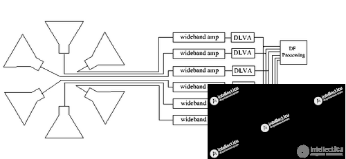
A schematic of a possible DF system, [ 18 ] : 101 using six antennas, [ 54 ] [ 55 ] is shown in the figure.
The signals received by the antennas are first amplified by a low-noise preamplifier and then detected by detector logarithmic video amplifiers (DLVAs). [ 56 ] [ 57 ] [ 58 ] The signal levels from the DLVAs are compared to determine the angle of arrival. By considering signal levels on a logarithmic scale, as the DLVAs provide, a large dynamic range is achieved [ 56 ] : 33 , and in addition, the direction-finding calculations are simplified when the main lobes of the antenna radiation patterns have a Gaussian characteristic, as shown previously.
A necessary step in DF analysis is determining the channel containing the largest signal, and this is accomplished using a high-speed comparator circuit. [ 44 ] In addition to the DF process, other signal properties can also be examined, such as pulse width, frequency, pulse repetition frequency (PRF), and modulation characteristics. [ 45 ] Comparator operation typically includes hysteresis to avoid jitter in the selection process when the direction of the incoming signal is such that two adjacent channels contain signals of similar amplitude.
Wideband amplifiers are often protected from local high-power sources (for example, aboard a ship) using input limiters and/or filters. Similarly, amplifiers may include notch filters to remove known but unwanted signals that could degrade the system's ability to process weaker signals. Some of these issues are discussed in the «RF circuit» section.
Часть 1 Determining the direction of radio emission, radio direction finding
Часть 2 Amplitude-comparison DF - Determining the direction of radio emission, radio

Comments