
Lecture
The Butterworth filter is one of the types of electronic filters. Filters of this class differ from others in their design method. The Butterworth filter is designed so that its amplitude-frequency response (magnitude response) is maximally flat in the passband.
Such filters were first described by the British engineer Stephen Butterworth . in the paper "On the Theory of Filter Amplifiers", published in Wireless Engineer magazine in 1930.
The magnitude response of the Butterworth filter is maximally flat in the passband and drops off to nearly zero in the stopband. When the frequency response of the Butterworth filter is plotted on a logarithmic scale, the amplitude drops toward minus infinity in the stopband. For a first-order filter, the magnitude response rolls off at −6 decibels per octave (-20 decibels per decade) (in fact, all first-order filters, regardless of type, are identical and have the same frequency response). For a second-order Butterworth filter, the magnitude response rolls off at −12 dB per octave, for a third-order filter — at −18 dB, and so on. The magnitude response of the Butterworth filter is a monotonically decreasing function of frequency.
The Butterworth filter is the only filter that preserves the shape of its magnitude response at higher orders (except for a steeper roll-off in the stopband), whereas many other filter types (Bessel filter, Chebyshev filter, elliptic filter) have different magnitude response shapes at different orders.
Compared to Chebyshev type I and II filters or the elliptic filter, the Butterworth filter has a more gradual roll-off and therefore must have a higher order (which is harder to implement) in order to achieve the required characteristics in the stopband. However, the Butterworth filter has a more linear phase response in the passband.
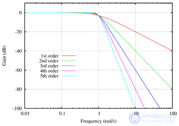
Log-magnitude response (Bode plot) for Butterworth low-pass filters of order 1 through 5. The slope of the response is —  dB/decade, where
  is the filter order.
As with all filters, when considering frequency characteristics a low-pass filter is used, from which a high-pass, band-pass, or band-stop (notch) filter can easily be obtained.
The magnitude response  of an -order Butterworth filter can be obtained from the transfer function
  :
:
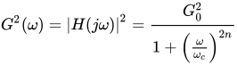
where
— filter order — cutoff frequency (the frequency at which the amplitude equals −3 dB)
 — DC gain (gain at zero frequency)
It is easy to see that for infinite values, the magnitude response becomes a rectangular function, and frequencies below the cutoff frequency will be passed with a gain of, while frequencies above the cutoff frequency will be fully suppressed. For finite values of the roll-off will be gradual.
Using the formal substitution  , let us write the expression
 in the form
 :
:
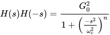
The poles of the transfer function lie on a circle of radius , equally spaced from each other in the left half-plane. That is, the transfer function of the Butterworth filter can be determined simply by finding the poles of its transfer function in the left half of the s-plane. The  -th pole is determined from the following expression:

from which

The transfer function can be written as:
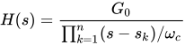
Similar reasoning applies to digital Butterworth filters, with the only difference being that the relations are written not for the s-plane, but for the z-plane.
The denominator of this transfer function is called the Butterworth polynomial.
Butterworth polynomials can be written in complex form, as shown above, but they are usually written as relations with real coefficients (complex-conjugate pairs are combined by multiplication). The polynomials are normalized to the cutoff frequency:  . The normalized Butterworth polynomials thus have the following canonical form:
 , for n — even
 , for n — odd
Below are the coefficients of the Butterworth polynomials for the first eight orders:
|
Polynomial coefficients  |
|---|---|
| 1 |  |
| 2 |  |
| 3 |  |
| 4 |  |
| 5 |  |
| 6 |  |
| 7 |  |
| 8 |  |
Taking and  , the derivative of the magnitude response with respect to frequency will look as follows:
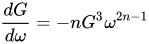
It decreases monotonically for all  since the gain is always positive. Thus, the magnitude response of the Butterworth filter has no ripples. Expanding the magnitude response in a series, we obtain:

In other words, all derivatives of the magnitude response with respect to frequency up to the  -th are equal to zero, from which "maximal flatness" follows.
Taking , let us find the slope of the log-magnitude response at high frequencies:
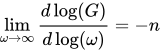
In decibels, the high-frequency asymptote has a slope of  dB/decade.
There are a number of different filter topologies used to implement linear analog filters. These circuits differ only in the values of their elements, while the structure remains unchanged.
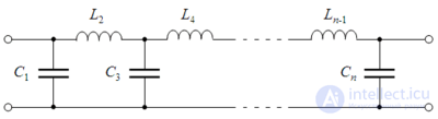
The Cauer topology uses passive elements (capacitors and inductors). A Butterworth filter with a given transfer function can be built in Cauer form 1. The -th element of the filter is given by the relation:
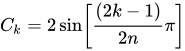 ; k odd
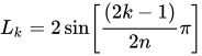 ; k even
The Sallen–Key topology uses active elements (operational amplifiers) in addition to passive ones. Each stage of a Sallen–Key circuit represents a part of the filter mathematically described by a pair of complex-conjugate poles. The complete filter is obtained by cascading all the stages in series. If a real pole occurs, it must be implemented separately, usually as an RC network, and included in the overall circuit.
The transfer function of each stage in a Sallen–Key circuit has the form:

The denominator must be one of the factors of the Butterworth polynomial. Taking , we obtain:

and

The last relation gives two unknowns, which can be chosen arbitrarily.
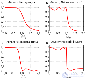
Comparison of the magnitude responses of 5th-order filters: Butterworth, Chebyshev type 1 and type 2, and elliptic
The figure shows the magnitude response of the Butterworth filter compared with other popular fifth-order linear filters.
The figure shows that the roll-off of the Butterworth filter's magnitude response is the slowest of the four, but it also has the smoothest magnitude response in the passband.
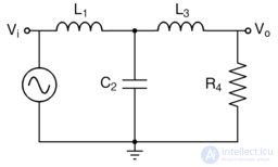
An analog Butterworth low-pass filter (Cauer topology) with cutoff frequency and the following element values:  farads,
  ohms,
ohms,  and
and  henries.
Consider an analog third-order Butterworth low-pass filter with farads, ohms,  and
and  henries. Denoting the impedance of the capacitors
  as
as  and the impedance of the inductors
  as
as  , where
  is a complex variable, and using the equations for circuit analysis, we obtain the following transfer function for this filter:

The magnitude response is given by the equation:

and the phase response is given by the equation:

Group delay is defined as minus the derivative of phase with respect to angular frequency and is a measure of the phase distortion of the signal at different frequencies. The log-magnitude response of such a filter has no ripples, either in the passband or in the stopband.
The plot of the magnitude of the transfer function on the complex plane clearly shows three poles in the left half-plane. The transfer function is fully determined by the location of these poles on the unit circle, symmetric about the real axis.
Replacing each inductor with a capacitor, and each capacitor with an inductor, gives a high-pass Butterworth filter.
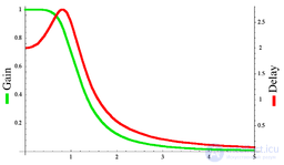
and group delay of a third-order Butterworth filter with cutoff frequency
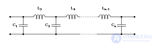
Butterworth filter using the Cauer topology
The Cauer topology uses passive components (shunt capacitors and series inductors) to implement a linear analog filter. A Butterworth filter with a given transfer function can be realized using Cauer 1 form. The k-th element is given by


Optionally, the filter can begin with a series inductor if desired, in which case Lk apply for k odd and Ck k even. These formulas can be usefully combined by defining Lk and C_k. Dividing the immittance by s gives kg. That is, kg equals k

These formulas apply to a doubly terminated filter (i.e., the source and load impedances are equal to unity) with ωc = 1. This filter prototype can be scaled for other impedance and frequency values. For a singly terminated filter (i.e., driven by an ideal voltage or current source), the element values are given by the expression

where

and


Voltage-driven filters must begin with a series element, while current-driven filters must begin with a shunt element. These forms are useful when designing diplexers and multiplexers.
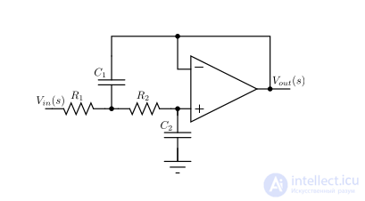
Sallen–Key topology
The Sallen–Key topology uses active and passive components (non-inverting buffers, usually operational amplifiers, resistors and capacitors) to implement a linear analog filter. Each Sallen–Key stage realizes a conjugate pole pair; the overall filter is realized by cascading all the stages in series. If a real pole exists (which happens when n is odd), it must be realized separately, usually as an RC circuit, and cascaded with the active stages.
For the second-order Sallen–Key circuit shown on the right, the transfer function is given by the expression

We want the denominator to be one of the quadratic factors of the Butterworth polynomial. Given that , this implies that

and

This leaves two undetermined component values, which can be chosen as desired.
Third- and fourth-order Sallen–Key-topology Butterworth low-pass filters using only a single operational amplifier are described by Huelsman, and other single-amplifier Butterworth filters of higher order are given by Jurišić et al.
Digital implementations of Butterworth and other filters are often based on the bilinear transform method or the matched Z-transform method, two different methods for discretizing an analog filter design. For all-pole filters such as the Butterworth, the matched Z-transform method is equivalent to the impulse-invariance method. At higher orders, digital filters become sensitive to quantization errors, so they are often computed as cascaded biquad sections plus one first- or third-order section for non-standard orders.

Comments