
Lecture
Tensor calculus is a branch of mathematics that studies tensors and tensor fields; it is divided into tensor algebra, which forms a core part of multilinear algebra, and tensor analysis, which studies differential operators on the algebra of tensor fields. Vector analysis and matrix algebra can be regarded as special branches of tensor calculus, since the notions of vector and matrix generalize into the notion of a tensor.
It is one of the principal tools of differential geometry. In this field, tensor calculus was developed by Tullio Levi-Civita and Gregorio Ricci-Curbastro (tensor calculus was formerly also called «Ricci calculus»). The calculus underwent especially rapid development in the early twentieth century owing to its wide application in relativistic physics.
It is the principal mathematical language in which the fundamental laws of such sciences as continuum mechanics, solid-state physics, electrodynamics, the theory of relativity, and its applications are formulated. From the standpoint of these applications, important directions within the calculus are the theory of tensor invariants and the theory of tensor functions.
In mathematics, a tensor is an algebraic object that describes a multilinear relationship between sets of algebraic objects associated with a vector space. Tensors can map between various objects such as vectors, scalars, and even other tensors. There are many types of tensors, including scalars and vectors (which are the simplest tensors), dual vectors, multilinear maps between vector spaces, and even certain operations such as the dot product. Tensors are defined independently of any basis, although they are often referred to by their components in a basis associated with a particular coordinate system; these components form an array that can be regarded as a multidimensional matrix.
Tensors became important in physics because they provide a concise mathematical framework for formulating and solving physical problems in such areas as mechanics (stress, elasticity, quantum mechanics, fluid mechanics, moment of inertia, ...), electrodynamics (the electromagnetic tensor, the Maxwell stress tensor, permittivity, magnetic susceptibility, ...), and general relativity (the stress-energy tensor, the curvature tensor, ...). Applications often examine situations in which a different tensor may arise at each point of an object; for example, the stress within an object may vary from one location to another. This leads to the concept of a tensor field. In some areas tensor fields are so ubiquitous that they are often simply called «tensors».
Tullio Levi-Civita and Gregorio Ricci-Curbastro popularized tensors in 1900 — building on the earlier work of Bernhard Riemann, Elwin Bruno Christoffel, and others — as part of the absolute differential calculus. This concept enabled an alternative formulation of the intrinsic differential geometry of a manifold in the form of the Riemann curvature tensor.
Despite their apparent differences, the various approaches to defining tensors describe the same geometric concept using different language and at different levels of abstraction.
A tensor can be represented as a (potentially multidimensional) array. Just as a vector in n-dimensional space is represented by a one-dimensional array with n components relative to a given basis, any tensor is represented relative to a basis by a multidimensional array. For example, a linear operator is represented in a basis as a two-dimensional square array n × n. The numbers in the multidimensional array are known as the components of the tensor. They are labeled by indices giving their position in the array, as lower and upper indices following the symbolic name of the tensor. For example, the components of a 2nd-order T tensor may be denoted as T ij, where i and j are indices running from 1 to n, or also as T i
j. Whether an index is written as a superscript or a subscript depends on the transformation properties of the tensor described below. Thus, while T ij and T i
jcan both be expressed as n by n matrices and are numerically related through index juggling, the difference in their transformation laws shows that it would be incorrect to add them together.
The total number of indices (m) needed to uniquely identify each component equals the dimension or the number of ways of the array, so a tensor is sometimes called an m-dimensional array or an m-way array. The total number of indices is also called the order, degree, or rank of the tensor, although the term «rank» usually has a different meaning in the context of matrices and tensors.
Just as the components of a vector change when the basis of the vector space changes, the components of a tensor also change under such a transformation. Each type of tensor is equipped with a transformation law that describes in detail how the components of the tensor respond to a change of basis. The components of a vector can respond to a change of basis in two different ways (see Covariance and contravariance of vectors), where the new basis vectors  are expressed in terms of the old basis vectors
  as,
as,
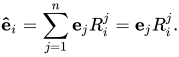
Here R j i are the elements of the change-of-basis matrix, and in the rightmost expression the summation sign has been dropped: this is the Einstein summation convention, which will be used throughout the article. [ Note 1 ] The components v i of the column vector v transform using the inverse of the matrix R,
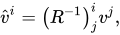
where the hat denotes the components in the new basis. This is called the contravariant transformation law, because the components of the vector transform by the inverse of the basis change. By contrast, the components w i of a covector (or row vector), w, transform using the matrix R itself,

This is called the covariant transformation law, because the components of the covector transform by the same matrix as the basis change. The components of a more general tensor transform by some combination of covariant and contravariant transformations, with one transformation law for each index. If the transformation matrix for an index is the inverse of the basis-transformation matrix, the index is called contravariant and is conventionally denoted by an upper index (a superscript). If the transformation matrix for an index is the basis transformation itself, the index is called covariant and is denoted by a lower index (a subscript).
As a simple example, the matrix of a linear operator relative to a basis is a rectangular arrayT that transforms, under a change of basis matrix  to
to  . For individual matrix elements this transformation law has the form
 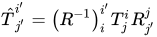 so the tensor corresponding to the matrix of a linear operator has one covariant and one contravariant index: it has type (1,1).
Combinations of covariant and contravariant components with the same index allow us to express geometric invariants. For example, the fact that a vector is the same object in different coordinate systems can be captured by the following equations, using the formulas defined above:
 ,
,
whereδjk is the Kronecker delta, which functions analogously to the identity matrix and has the effect of renaming indices (in this example j to k). This reveals several features of component notation: the ability to reorder terms at will (commutativity), the need to use different indices when working with several objects in a single expression, the ability to rename indices, and the way in which contravariant and covariant tensors combine so that all instances of the transformation matrix and its inverse cancel out, so that expressions of the type
  can be seen at once to be geometrically identical in all coordinate systems.
Similarly, a linear operator, viewed as a geometric object, does not actually depend on a basis: it is simply a linear map that takes a vector as its argument and produces another vector. The transformation law describing how the component matrix of a linear operator changes with the basis is consistent with the transformation law for a contravariant vector, so that the action of the linear operator on a contravariant vector is represented in coordinates as the matrix product of their respective coordinate representations. That is, the components  are given by
 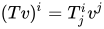 . These components transform contravariantly, since
( 
The transformation law for a tensor of order p + q with p contravariant indices and q covariant indices is thus given as,



Here primed indices denote components in the new coordinates, and unprimed indices denote components in the old coordinates. Such a tensor is said to have order, or type ( p , q ). The terms «order», «type», «rank», «valence», and «degree» are sometimes used for the same concept. Here the term «order» or «total order» will be used for the overall dimensionality of the array (or its generalization in other definitions), p + q in the preceding example, while the term «type» will be used for the pair giving the number of contravariant and covariant indices. A tensor of type ( p , q ) is also called a ( p , q )-tensor for short.
This discussion motivates the following formal definition:
Definition. A tensor of type ( p , q ) is an assignment of a multidimensional array
to every basis f = ( e 1 , ..., e n ) of an n -dimensional vector space, such that if we apply a change of basis
then the multidimensional array obeys the transformation law


The definition of a tensor as a multidimensional array satisfying the transformation law goes back to the work of Ricci.
An equivalent definition of a tensor uses representations of the general linear group. There is an action of the general linear group on the set of all ordered bases of an n -dimensional vector space. If  is an ordered basis, and
  is an invertible
  matrix, then the action is given by

Let F be the set of all ordered bases. Then F is a principal homogeneous space for GL( n ). Let W be a vector space, and letρ be a representation of GL( n ) on W (that is, a group homomorphism
  ). Then a tensor of typeρis an equivariant map
  . Equivariance here means that

When ρ is a tensor representation of the general linear group, this yields the usual definition of tensors as multidimensional arrays. This definition is often used to describe tensors on manifolds, and it generalizes readily to other groups.
A drawback of defining a tensor using the multidimensional-array approach is that it is not evident from the definition that the object being defined is truly independent of the basis, as is expected of an intrinsically geometric object. Although it can be shown that the transformation laws do indeed guarantee basis independence, a more intrinsic definition is sometimes preferable. One approach, common in differential geometry, is to define tensors relative to a fixed (finite-dimensional) vector space V, which is usually taken to be a particular vector space of some geometric significance, such as the tangent space of a manifold. [ 8 ] In this approach, a tensor of type ( p , q ) T is defined as a multilinear map,

where V ∗ is the corresponding dual space of covectors, linear in each of its arguments. The above assumes that V is a vector space over the real numbers, . More generally, V can be taken over any field F (for example, the complex numbers), replacing F as the range of the multilinear maps.
Applying the multilinear map T of type ( p , q ) to a basis { e j } for V and the canonical cobasis { ε i } for V ∗ ,

This yields a ( p + q ) -dimensional array of components. A different choice of basis will give different components. But since T is linear in all of its arguments, the components satisfy the tensor transformation law used in the definition of the multilinear-array approach. The multidimensional array of components of T thus forms a tensor according to this definition. Moreover, such an array can be realized as the components of some multilinear map T. This motivates regarding multilinear maps as the intrinsic objects underlying tensors.
When regarding a tensor as a multilinear map, it is conventional to identify the double dual V ∗∗ of a vector space V, i.e., the space of linear functionals on the dual vector space V ∗, with the vector space V. There is always a natural linear map from V into its double dual, given by evaluating a linear form in V ∗ at a vector in V. This linear map is an isomorphism in finite dimensions, and it is often then convenient to identify V with its double dual.
For some mathematical applications a more abstract approach is sometimes useful. This can be achieved by defining tensors in terms of elements of tensor products of vector spaces, which are in turn defined via a universal property, as explained here and here.
Tensor of type ( p , q ) is defined in this context as an element of the tensor product of vector spaces ,

A basis v i for V and a basis w j for W naturally induce a basis v i ⊗ w j of the tensor product V ⊗ W. The components of the tensor T are the coefficients of the tensor relative to the basis obtained from the basis { ei } for V and its dual basis { ε j } , i.e.

Using the properties of the tensor product, one can show that these components satisfy the transformation law for a tensor of type ( p , q ). Moreover, the universal property of the tensor product gives a one-to-one correspondence between tensors defined in this way and tensors defined as multilinear maps.
This 1-to-1 correspondence can be achieved as follows, since in the finite-dimensional case there is a canonical isomorphism between a vector space and its double dual space:

The last line uses the universal property of the tensor product, namely that there is a correspondence between maps from 
 .
.
Tensor products can be defined with great generality – for example, using arbitrary modules over a ring. In principle, one could define a «tensor» simply as an element of any tensor product. However, in the mathematical literature the term « tensor » is usually reserved for an element of a tensor product of any number of copies of a single vector space V and its dual, as indicated above.
This discussion of tensors has so far assumed the spaces involved are finite-dimensional, where the tensor spaces obtained by each of these constructions are naturally isomorphic. [ Note 2 ] Constructions of tensor spaces based on the tensor product and on multilinear maps can be generalized, essentially unchanged, to vector bundles or coherent sheaves. For infinite-dimensional vector spaces, inequivalent topologies give rise to inequivalent notions of tensor, and these various isomorphisms may or may not hold depending on exactly what is meant by a tensor (see topological tensor product). In some applications it is the tensor product of Hilbert spaces that is intended, whose properties are closest to the finite-dimensional case. A more modern viewpoint is that it is the structure of tensors as a symmetric monoidal category that encodes their most important properties, rather than any particular model of these categories.
In many applications, especially in differential geometry and physics, it is natural to consider a tensor with components that are functions of a point in space. This was the setting of Ricci's original work. In modern mathematical terminology such an object is called a tensor field, often simply referred to as a tensor.
In this context, a coordinate basis is often chosen for the tangent vector space. The transformation law can then be expressed in terms of partial derivatives of the coordinate functions,
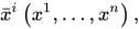
defining the coordinate transformation,

The concepts of later tensor analysis arose from the work of Carl Friedrich Gauss in differential geometry, and the formulation was heavily influenced by the theory of algebraic forms and invariants developed in the mid-nineteenth century. The word «tensor» itself was introduced in 1846 by William Rowan Hamilton to describe something different from what is now meant by a tensor. [ Note 3 ] Gibbs introduced dyadic and polyadic algebra, which are also tensors in the modern sense. The modern usage was introduced by Woldemar Voigt in 1898.
Tensor calculus was developed around 1890 by Gregorio Ricci-Curbastro under the name «absolute differential calculus» and originally presented in 1892. It became accessible to many mathematicians after the 1900 publication of Ricci-Curbastro and Tullio Levi-Civita's classic text, Methods of Absolute Differential Calculus and Their Applications (Méthodes de calcul différentiel absolu et leurs applications). In Ricci's notation he refers to «systems» with covariant and contravariant components, which in the modern sense are known as tensor fields. In the 20th century the subject became known as tensor analysis and gained wider acceptance with the introduction of Albert Einstein's general theory of relativity around 1915. General relativity is formulated entirely in the language of tensors. Einstein learned about them with great difficulty from the geometer Marcel Grossmann. Levi-Civita then began a correspondence with Einstein to correct mistakes that Einstein had made in his use of tensor analysis. The correspondence continued from 1915 to 1917 and was marked by mutual respect:
I admire the elegance of your method of computation; it must be nice to ride through these fields upon the horse of true mathematics while the like of us have to make our way laboriously on foot.
— Albert Einstein
Tensors and tensor fields have also proven useful in other fields, such as continuum mechanics. Some well-known examples of tensors in differential geometry are quadratic forms, such as metric tensors and the Riemann curvature tensor. The exterior algebra of Hermann Grassmann from the mid-nineteenth century is itself a tensor theory, and a highly geometric one, but it took some time before it came to be seen, along with the theory of differential forms, as naturally unified with tensor calculus. The work of Élie Cartan made differential forms one of the basic kinds of tensors used in mathematics, and Hassler Whitney popularized the tensor product.
Beginning around the 1920s, it was recognized that tensors play a fundamental role in algebraic topology (for example, in the Künneth theorem). Accordingly, there are types of tensors at work in many branches of abstract algebra, particularly in homological algebra and representation theory. Multilinear algebra can be developed with greater generality than for scalars coming from a field. For example, scalars may come from a ring. But then the theory is less geometric, and the computations are more technical and less algorithmic. Tensors have been generalized within category theory by means of the concept of a monoidal category since the 1960s.
An elementary example of a map described as a tensor is the dot product, which maps two vectors to a scalar. A more elaborate example is the Cauchy stress tensor T, which takes a directional unit vector v as input and maps it to the stress vector T ( v ), which is the force (per unit area) exerted by the material on the negative side of the plane orthogonal to v, against the material on the positive side of the plane, thereby expressing a relationship between these two vectors, shown in the figure (right). The vector cross-symmetric product, where two vectors are mapped to a third, is not strictly speaking a tensor, since it changes sign under those transformations that reverse the orientation of the coordinate system. The fully antisymmetric symbol  nevertheless makes it convenient to handle the cross product in identically oriented three-dimensional coordinate systems.
This table gives important examples of tensors on vector spaces and tensor fields on manifolds. Tensors are classified according to their type ( n , m ), where n is the number of contravariant indices, m is the number of covariant indices, and n + m gives the total order of the tensor. For example, a bilinear form is the same thing as a (0, 2)-tensor; the dot product is an example of a (0, 2)-tensor, but not every (0, 2)-tensor is a dot product. In a (0, M )-entry of the table, M denotes the dimension of the underlying vector space or manifold, since a separate index is needed for each dimension of the space in order to obtain a maximally covariant antisymmetric tensor.
| m | ||||||||
|---|---|---|---|---|---|---|---|---|
| 0 | 1 | 2 | 3 | ⋯ | M | ⋯ | ||
| n | 0 | Scalar, e.g. scalar curvature | Covector, linear functional, 1-form, e.g. dipole moment, gradient of a scalar field | Bilinear form, e.g. dot product, quadrupole moment, metric tensor, Ricci curvature, 2-form, symplectic form | 3-form, e.g. octupole moment | For example, an M-form, i.e. a volume form. | ||
| 1 | Euclidean vector | Linear transformation, Kronecker delta | e.g. cross product in three dimensions | e.g. Riemann curvature tensor | ||||
| 2 | Inverse metric tensor, bivector, e.g. Poisson structure | e.g. elasticity tensor | ||||||
| ⋮ | ||||||||
| N | Multivector | |||||||
| ⋮ |
Raising the index of an ( n , m )-tensor produces an ( n + 1, m − 1)-tensor; this corresponds to moving diagonally down and to the left in the table. Symmetrically, lowering an index corresponds to moving diagonally up and to the right in the table. Contracting an upper index with a lower index of an ( n , m )-tensor produces an ( n − 1, m − 1)-tensor; this corresponds to moving diagonally up and to the left in the table.
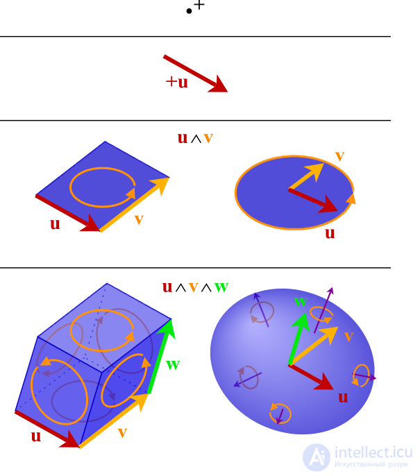
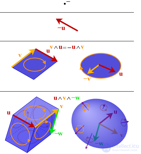
Assuming a basis of a real vector space, e.g., a coordinate system in the ambient space, a tensor can be represented as an organized multidimensional array of numerical values with respect to this particular basis. Changing the basis transforms the values in the array in a characteristic way, which allows tensors to be defined as objects adhering to this transformational behavior. For example, there are invariants of tensors that must be preserved under any change of basis, thereby making only certain multidimensional arrays of numbers a tensor. Compare this to the array representingnot being a tensor, on account of changing sign under orientation-reversing transformations.
Since the components of vectors and their duals transform differently under changes of their dual bases, there is a covariant and/or contravariant transformation law that relates the arrays representing a tensor with respect to one basis and the arrays with respect to another. The numbers, respectively, of vectors: n (contravariant indices) and dual vectors: m (covariant indices) on the input and output of the tensor determine the type (or valence) of the tensor, a pair of natural numbers ( n , m ), which determine the precise form of the transformation law. The order of the tensor equals the sum of these two numbers.
The order (also degree orrank ) of a tensor is thus the sum of the orders of its arguments plus the order of the resulting tensor. This is also the dimensionality of the array of numbers needed to represent the tensor with respect to a given basis, or, equivalently, the number of indices needed to label each component in that array. For example, in a fixed basis, a standard linear map that maps a vector to a vector is represented by a matrix (a two-dimensional array) and is therefore a tensor of order 2. A simple vector can be represented as a one-dimensional array and is therefore a tensor of order 1. Scalars are simple numbers and are thus tensors of order 0. Thus, the tensor representing the dot product, taking two vectors and yielding a scalar as a result, has order2 + 0 = 2, the same as the stress tensor, taking one vector and returning another-symbol, mapping two vectors to one vector, would have order 2 + 1 = 3.
The collection of tensors on a vector space and its dual space form a tensor algebra , which admits products of arbitrary tensors. Simple applications of order-2 tensors, which can be represented as a square matrix, can be solved by a clever arrangement of transposed vectors and application of the rules of matrix multiplication, but the tensor product should not be confused with this.
There are several notational systems used to describe tensors and perform computations involving them.
Ricci calculus — is the modern formalism and notation for tensor indices: denoting inner and outer products , covariance and contravariance , summation of tensor components, symmetry and antisymmetry , and partial and covariant derivatives .
The Einstein summation convention dispenses with writing summation signs, leaving the summation implicit. Any repeated index symbol is summed over: if the index i is used twice in a given term of a tensor expression, this means the term must be summed over all i . Several different pairs of indices may be summed in this way.
Penrose graphical notation — is a diagrammatic notation that replaces tensor symbols with shapes, and their indices — with lines and curves. It is independent of basis elements and requires no symbols for indices.
Abstract index notation — is a way of writing tensors such that the indices are no longer treated as numerical but rather as indeterminates . This notation reflects the expressiveness of indices and the basis independence of index-free notation.
The component-free treatment of tensors uses notation that emphasizes that tensors do not rely on any basis, and defines them in terms of the tensor product of vector spaces .
There are several operations on tensors that again produce a tensor. The linear nature of a tensor implies that two tensors of the same type can be added together, and that tensors can be multiplied by a scalar with results analogous to scaling a vector . On components, these operations are simply performed componentwise. These operations do not change the type of the tensor; but there are also operations that produce a tensor of a different type.
The tensor product takes two tensors, S and T , and produces a new tensor, S ⊗ T , whose order is the sum of the orders of the original tensors. When described as multilinear maps, the tensor product simply multiplies the two tensors, i.e. which again produces a map that is linear in all its arguments. On components, the effect is to multiply the components of the two input tensors pairwise, i.e.
  If S has type ( l , k ), and T has type ( n , m ) , then the tensor product S ⊗ T has type ( l + n , k + m ) .
Tensor contraction is an operation that reduces a tensor of type ( n , m ) to a tensor of type ( n − 1, m − 1) , a special case of which is the trace . It thereby reduces the total order of the tensor by two. The operation is achieved by summing components for which one specified contravariant index matches one specified covariant index, to obtain a new component. Components for which these two indices differ are discarded. For example, a (1, 1) -tensor can be contracted to a scalar through
 , where summation is again implied. When a (1, 1) -tensor is interpreted as a linear map, this operation is known as the trace .
Contraction is often used in conjunction with the tensor product to contract an index from each tensor.
Contraction can also be understood using the definition of a tensor as an element of the tensor product of copies of the space V with the space V ∗, first by decomposing the tensor into a linear combination of simple tensors, and then applying a factor from V ∗ to a factor from V . For example, the tensor can be written as a linear combination

The contraction of T on the first and last slots is then a vector

In a vector space with a dot product (also known as a metric ) g , the term contraction is used for removing two contravariant or two covariant indices by forming a trace with the metric tensor or its inverse. For example, a (2, 0) -tensor can be contracted to a scalar through
 (again assuming the summation convention).
When a vector space is equipped with a nondegenerate bilinear form (or metric tensor , as it is often called in this context), operations can be defined that convert a contravariant (upper) index into a covariant (lower) index and vice versa. The metric tensor is a (symmetric) ( 0, 2) -tensor; it is thus possible to contract an upper index of a tensor with one of the lower indices of the metric tensor in the product. This produces a new tensor with the same index structure as the previous tensor, but with a lower index, usually shown in the same position as the contracted upper index. This operation is quite graphically known as lowering an index .
Conversely, the inverse operation can be defined and is called raising an index . This is equivalent to a similar contraction on the product with a (2, 0) -tensor. This inverse metric tensor has components that are the matrix inverse of the components of the metric tensor.
Continuum mechanics provides important examples. The stresses inside a solid body or fluid [ 28 ] are described by a tensor field. The stress tensor and the strain tensor are second-order tensor fields and are related, in a general linear elastic material, by a fourth-order elasticity tensor field . In detail, the tensor quantifying the stress in a three-dimensional solid object has components that can be conveniently represented as a 3 × 3 array. The three faces of a cubic infinitesimal volume segment of the solid body are subject to some given force. The force's vector components also number three. Thus, describing the stress in this cubic infinitesimal segment requires 3 × 3, or 9 components. Within this solid body there is an entire mass of different stress quantities, each of which requires 9 quantities to describe. Thus a second-order tensor is required.
If a particular surface element within the material is singled out, the material on one side of the surface will exert a force on the other side. In general, this force will not be orthogonal to the surface, but will depend linearly on the surface's orientation. This is described by a tensor of type ( 2, 0) in linear elasticity, or, more precisely, by a tensor field of type (2, 0) , since the stresses may vary from point to point.
Common areas of application include:
The notion of a second-order tensor is often conflated with that of a matrix. Higher-order tensors, however, capture ideas important in science and engineering, as has been shown time and again in numerous fields as they developed. This occurs, for example, in the field of computer vision , where the trifocal tensor generalizes the fundamental matrix .
The field of nonlinear optics studies changes to the polarization density of a material under extreme electric fields. The generated polarization waves are related to the generating electric fields through the nonlinear susceptibility tensor. If the polarization P is not linearly proportional to the electric field E , the medium is called nonlinear . To a good approximation (for sufficiently weak fields, assuming no permanent dipole moments are present), P is given by a Taylor series in E, whose coefficients are the nonlinear susceptibilities:

Here is the linear susceptibility,
 gives the Pockels effect and second-harmonic generation, and
 gives the Kerr effect . This expansion shows how higher-order tensors arise naturally in the subject.
The properties of tensors , especially tensor decomposition , have enabled their use in machine learning for embedding multidimensional data in artificial neural networks . This notion of a tensor differs substantially from that in other areas of mathematics and physics, in the sense that a tensor is usually regarded as a numerical quantity in a fixed basis, and the dimensionality of the spaces along the tensor's different axes need not be the same.
The vector spaces of a tensor product need not be the same, and sometimes elements of such a more general tensor product are called «tensors». For example, an element of the tensor product space V ⊗ W is a «tensor» of second order in this more general sense, [ 29 ] and a tensor of order d can likewise be defined as an element of the tensor product of d different vector spaces. [ 30 ] A tensor of type ( n , m ) in the sense defined earlier is also a tensor of order n + m in this more general sense. The notion of tensor product can be extended to arbitrary modules over a ring .
The notion of a tensor can be generalized in various ways to infinite dimensions . For example, one way is through the tensor product of Hilbert spaces . [ 31 ] Another way of generalizing the idea of a tensor, common in nonlinear analysis , is through the definition of multilinear maps , where instead of using finite-dimensional vector spaces and their algebraic dual spaces, infinite-dimensional Banach spaces and their continuous dual spaces are used. [ 32 ] Thus, tensors naturally exist on Banach manifolds [ 33 ] and Fréchet manifolds .
Suppose a homogeneous medium fills R 3 , so that the density of the medium is described by a single scalar value ρ in kg⋅m −3 . The mass in kg of a region Ω is obtained by multiplying ρ by the volume of the region Ω , or, equivalently, by integrating the constant ρ over the region:
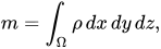
where the Cartesian coordinates x , y , z are measured in m . If the unit of length is changed to cm , the numerical values of the coordinate functions must be rescaled by a factor of 100:

The numerical value of the density ρ must then also be rescaled by 100−3 m 3 /cm 3 to compensate, so that the numerical value of the mass in kg is still given by the integral of . Thusρ
 (in units of kg⋅cm −3 ).
More generally, if the Cartesian coordinates x , y , z undergo a linear transformation, then the numerical value of the density ρ must change by a factor equal to the inverse of the absolute value of the determinant of the coordinate transformation, so that the integral remains invariant, by the change-of-variables formula for integration. Such a quantity, which scales by the inverse of the absolute value of the determinant of the coordinate transition map, is called a scalar density . To model a non-constant density, ρ is a function of the variables x , y , z ( a scalar field ), and under a curvilinear change of coordinates it transforms by the inverse of the Jacobian of the coordinate change. For more on the intrinsic meaning, see Density on a manifold .
A tensor density transforms like a tensor under a change of coordinates, except that it additionally acquires a factor of the absolute value of the determinant of the coordinate transition: [ 34 ]

Here w is called the weight. In general, any tensor multiplied by a power of this function or its absolute value is called a tensor density or a weighted tensor. An example of a tensor density is the current density of electromagnetism .
Under an affine change of coordinates, a tensor transforms by the linear part of the transformation itself (or its inverse) on each index. These arise from rational representations of the general linear group. But this is not quite the most general linear transformation law that such an object can have: tensor densities are non-rational, yet are still semisimple representations. A further class of transformations comes from the logarithmic representation of the general linear group, a reducible but not semisimple representation, [ 37 ], consisting of ( x , y ) ∈ R 2 with the transformation law

The transformation law for a tensor behaves as a functor on the category of admissible coordinate systems under general linear transformations (or other transformations within some class, such as local diffeomorphisms ). This makes a tensor a special case of a geometric object, in the technical sense that it is a function of the coordinate system, transforming functorially under a change of coordinates. Examples of objects obeying more general kinds of transformation laws are jets and, more generally still, natural bundles .
When passing from one orthonormal basis (called a frame ) to another by a rotation, the components of a tensor transform by that same rotation. This transformation does not depend on the path taken through the space of frames. However, the space of frames is not simply connected (see orientation entanglement and the plate trick ): in the space of frames there exist continuous paths with the same initial and final configurations that cannot be deformed into one another. One can attach an additional discrete invariant to each frame that incorporates this path dependence and that turns out to (locally) take the values ±1. A spinor is an object that transforms like a tensor under rotations of the frame, except for a possible sign, which is determined by the value of this discrete invariant.
Spinors are elements of the spin representation of the rotation group, whereas tensors are elements of its tensor representations . Other classical groups have tensor representations, as well as tensors compatible with the group, but all noncompact classical groups also have infinite-dimensional unitary representations.




Comments