
Lecture
Spline (from Eng. spline, from [flat] spline — a flexible batten, a flexible loft rail — a strip of metal used for drawing curved lines) is a function in mathematics whose domain is divided into a finite number of intervals, on each of which it coincides with some algebraic polynomial. The highest of the degrees of the polynomials used is called the degree of the spline. The difference between the degree of the spline and the resulting smoothness is called the defect of the spline. For example, a continuous polyline is a spline of degree 1 and defect 1. In the modern sense, splines are solutions of multipoint boundary value problems obtained by grid methods.
In other words, a spline is a piecewise-defined function, that is, a collection of several functions, each defined on some set of argument values, with these sets being pairwise disjoint.
Splines have numerous applications both in mathematical theory and in applied mathematics (in particular, in various computational programs). In particular, splines of two variables are widely used to define surfaces in various computer modeling systems. Splines of two arguments are called bi-splines (for example, the bicubic spline), which are two-dimensional splines used to model surfaces. They are often confused with B-splines (basis splines), which are one-dimensional and, in linear combination, form curves — a framework for «stretching» surfaces over. Basis splines can also be combined into a three-dimensional construction for modeling solid bodies.
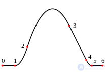
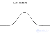
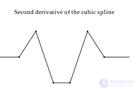
The term spline (Eng. spline) originally referred to a flexible metal ruler — a universal batten , which draftsmen used to connect points on a drawing with a smooth curve, that is, to carry out interpolation graphically.
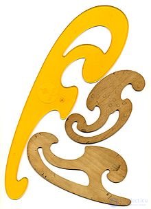
Moreover, the curve that describes the deformation of a flexible ruler fixed at individual points is itself a spline. Thus, there is a physical model of the spline function (or, conversely, the spline function is a mathematical model of the flexible ruler). An intuitive approach to using piecewise functions in approximation problems has appeared in mathematics for a long time. The physical model known as the mechanical analogy of a spline is a multi-support beam that experiences no external load, whose deformations are caused by internal reactions to given displacements of the supports at fixed nodes. Mathematically, this model is described by the differential equation of beam deformation and is a multipoint boundary value problem, for the solution of which a grid method known at the time was applied, yielding a solution of exactly the form known today as a spline. However, as the Soviet scientist Nikolai Korneichuk noted, the incursion of splines into approximation theory occurred because of the interpolation problem, owing to their good computational and approximation properties. Splines have exceptionally good approximation properties, versatility, and provide simplicity in implementing the computational algorithms based on them. At the same time, the algorithms for constructing splines coincide with the algorithm of the finite element method, which is the main industrial method of strength analysis in computer-aided design (CAD) systems.
The theory of spline interpolation, and the term spline itself, date back to a 1946 paper by Isaac Jacob Schoenberg. Its development was especially intensive in the 1950s-1970s. Today, CAD systems remain the traditional application area for interpolation splines. However, the potential of splines is considerably wider than merely describing certain curves. In the real world, a great many physical processes are, by their very nature, splines. In mechanics, examples include the deformation of a flexible plate or rod fixed at individual points, or the trajectory of a body when the force acting on it changes in a stepwise manner (the trajectory of an artificial space object with powered and coasting segments, or the trajectory of an aircraft under stepwise changes in engine thrust and wing profile, and so on). In thermodynamics, this is heat transfer along a rod made up of segments with different thermal conductivities. In chemistry, it is diffusion through layers of different substances. In electricity, it is the propagation of electromagnetic fields through inhomogeneous media. That is, a spline is not a contrived mathematical abstraction but, in many cases, the solution of differential equations describing quite real physical processes.
Let us begin our discussion of splines with the definition of an algebraic spline. A function  , defined and continuous on an interval
  , is called a polynomial spline of order
  with knots
  if, on each of the subintervals
  , is an algebraic polynomial of degree not exceeding , while at each of the points
  some derivative
  may have a discontinuity. If the functions
  are continuous at the points , while the derivatives
  are discontinuous at the points , then the numbers are called the defects of the spline. The set
  is called the knot mesh of the spline, and the points are called knots, points of contact, or splicing points of the spline.
As follows from the definition, to construct a spline consisting of  segments, one must find, for each segment — a polynomial of degree — such numerical parameter values as will ensure continuity at the knots both of the function itself and of the required derivatives. In total,
  parameters must be determined. Taking into account the interpolation condition and the continuity of the first two derivatives, determining the parameters reduces to solving a system consisting of
  linear equations. As a rule, the coefficient values for the polynomial segments are not computed directly.
To determine an interpolation spline with a continuous first derivative, it is enough to compute the value of the first derivative at the knots. The way in which the derivatives at the spline's knots are determined gives rise to a wide variety of interpolation splines. Often the derivatives are determined not as constants but as some functions of the interpolated function and the interpolation mesh.
If the value of the first derivative at the knots is computed from the condition that the second derivative be continuous (by solving a system made up of n linear equations), the spline will have two continuous derivatives. Such a method of constructing a spline, and the spline itself, is called global, since determining each of its coefficients takes into account the entire set of interpolation knots.
In other cases, determining an individual coefficient takes into account only the nearest interpolation knots, and such construction methods, as well as the splines themselves, are called local. The parameters of a segment of such a spline can be determined independently of the other segments.
A simple condition for constructing a local spline segment is that the polynomial equal the corresponding values of the interpolated function at the ends of the intervals.

For the simplest spline — a polyline — this condition alone is quite sufficient. The two coefficients of the line are uniquely determined from two equations. Such a spline is local. For higher-degree polynomials, additional conditions must be added so that the total number of equations equals the number of polynomial coefficients. Thus, for a degree-3 spline, such a condition is that the first derivative at the ends of the interval equal some value, determined in the same way for adjacent segments (in formulas (2), via an approximate value of the function's derivative).

A system of 4 equations
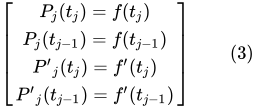
makes it possible to uniquely determine the four coefficients of the polynomial. For a degree-5 polynomial, a condition requiring equality of the second derivative at the ends of the interval must be added, and so on. From this it should be clear why splines are built mainly from odd-degree polynomials (with an even number of coefficients).
For even-degree polynomials, when assembling system (3):
which is why, for a degree-2 polynomial, it is impossible to achieve equality of the first derivative at the junction points, and for a degree-4 polynomial — of the second derivative, and so on. To construct splines of even degree, additional conditions are artificially added to form a system of equations similar to (3). If the derivatives of the spline's polynomial are determined in the same way as the corresponding derivatives of the interpolated function, the spline is called Hermite.

There exist local methods for constructing Bessel and Akima splines, B-splines. Generally, when splines are discussed, what is meant is splines built from algebraic polynomials. It is precisely to these that the definition given above applies. These are also the most thoroughly studied splines. However, a spline can consist of segments of functions of any class. Obviously, for any class of functions from which a spline is made up, the definition given at the beginning of this article does not entirely apply. For example, if a spline consists of segments of an exponential function, the notion of the spline's defect loses its meaning. Although the number of continuous derivatives remains an important characteristic. Constructing a spline whose segments are discontinuous functions (rational functions, Padé functions) goes somewhat beyond the spline concept, since one of the main advantages of splines is their smoothness. If such constructions are extended arbitrarily, the distinction between splines and piecewise functions is erased. Another advantage of splines is computational efficiency. Excessive complication of the segments substantially reduces the advantage of splines over classical functions.
Splines are characterized by the following features: a spline consists of segments — functions of a single class that differ only in their parameters; certain conditions are imposed on adjacent segments at the junction points, which reduce to continuity of the values and of some of the first derivatives. Splines are a branch of applied mathematics that is developing intensively. The Internet contains an extensive bibliography on splines (the Spline Bibliography Database, SBD).
As noted above, there is a large number of constructions called splines. It is therefore necessary to introduce a certain classification into this variety, with the aim of identifying the features that make it possible to choose splines suitable for a specific applied problem.
Purpose of splines. By purpose, three main groups of splines can be distinguished: «interpolation splines» or «functional splines» — passing exactly through given points; «smoothing splines» — passing through given points while taking into account the errors in their determination; and «correlation splines» — passing through a correlated set of points and reflecting its overall trend (regression). Interpolation and functional splines are used in geometric modeling problems, for example, to define the hull lines of ships and aircraft. Smoothing splines are most often used to describe the relationships found in physical experiments with a known measurement error. Correlation splines are used as nonlinear regression curves, the simplest of which can be considered the description of a relationship by a step function or a piecewise-linear function (splines of degree zero and one).
Shape of the spline's segments. The fact that a spline consists of segments of the same kind is one of the key features that distinguishes it from other piecewise functions. However, there are combined splines consisting of segments of different types of splines.
The best-known splines are those made up of segments that are algebraic polynomials not exceeding a given degree. As a rule, these are cubic polynomials or polynomials of odd degree: first, third (cubic), or fifth degree. Higher degrees are rarely used because of the increased complexity of the calculations and the difficulties described in the previous section. Their main advantage is the simplicity of computation and analysis. Their drawback is that relatively few real physical processes correspond to this kind of dependence.
Exponential splines. If a flexible metal ruler fixed at the knots is stretched taut, the solution of the differential equation will not be an algebraic polynomial but an exponential function. For this reason, such splines are also called tensioned. An exponential function describes many physical processes in dynamical systems. Its drawback is the laboriousness of the calculations.
By mechanical analogy with the metal ruler, which represents a computational model of a beam, one obtains splines of variable stiffness, described in the works of V. F. Snigirev and A. P. Pavlenko. Originally, such splines were called degenerate or logarithmic, since the solution of the underlying spline differential equation, representing a spline segment, contains natural logarithmic functions. The stiffness in them can act either as a weighting function, if it is given in advance, or as a control function, which is found from the condition of minimizing the energy functional of the operator of the underlying spline equation, analogous to the total potential energy of deformation of the ruler (beam). The stiffness function makes it possible to control the shape of the spline. When the stiffness function is a control function, such splines are called minimum-stiffness splines.
Trigonometric splines are those whose segments are described by trigonometric polynomials. They have fairly complex computational expressions. More than fifty different kinds of spline segments are described in the works of B. A. Popov.
There also exist rational splines and Padé splines. Their distinguishing feature is the possibility of discontinuities in the derivatives on the segments while remaining continuous at the knots. M. Anserme constructs fractional splines, in which the segments are defined using the gamma function.
The choice of a particular kind of segment is based on the specific conditions of the problem and the constraints of implementation. As a rule, the main requirement is to achieve the required interpolation accuracy at an acceptable cost in time and implementation resources. A well-chosen segment type that matches the nature of the process makes it possible to reduce computation time and the required amount of memory.
Number of segments. Obviously, the minimum number of segments is one. The classical definition of a spline limits the number of segments to a fixed number over a finite interval. However, splines with an infinite number of segments can also be constructed, and in practice these are methods and algorithms that do not need information about a specific number of segments[which?]. Representatives of these splines are the cardinal splines studied by Schoenberg. Local splines are better suited for constructing splines with an unlimited number of segments.
Segment width. Splines with equal segment widths deserve special mention. This makes it possible to considerably simplify the computational expressions, speed up the algorithms, and reduce implementation costs. A further simplification can be achieved by using segments with widths that are multiples of one another. There exist splines with zero-width segments (de Boor). This leads to multiplicity of the knots and to the possibility of approximating discontinuous functions with splines whose segments remain continuous. The computational expressions are obtained by taking limits. Splines can also have segments of infinite width. Such segments must be the outermost ones. This sometimes makes it possible to naturally specify the boundary conditions. Strictly speaking, the segment width depends on the choice of parameter — the argument of the spline function — and this requires solving a separate parametrization problem. The ideal choice of parameter is the arc length of the interpolated function, which is not always known, so there are many ways of solving this problem. The most common approach is parametrization by chords.
Segment junction conditions. This is another important feature that distinguishes splines. When splines are discussed, it is generally assumed that the segments join smoothly, that is, continuity of the values and of the first derivative is ensured. The notion of spline defect is related to the number of continuous derivatives possessed by a segment function of a given kind, and the number of derivatives whose continuity is guaranteed at the knots. An exponential function or a sinusoid has an infinite number of derivatives. For them, this notion has no meaning. It is therefore more convenient to speak directly of the number of derivatives whose continuity is guaranteed at the spline's knots. In practice, what is meant is continuity of the values and of the first, or at most the second, derivative. A discontinuity in the second or higher derivatives is not visually noticeable, so it is rarely taken into account. It is clear that the first derivative at the junction points can be specified in various ways. Two approaches are most common. The value of the first derivative is chosen so as to ensure continuity of the second derivative (global cubic splines of minimal defect). The first derivative equals the first derivative of the interpolated function (possibly approximately) in Hermite splines.
Boundary conditions. There are 4 types of classical boundary conditions and a number of non-classical ones. If a spline has a limited number of segments, then, naturally, it has no outer segments to the left and right, so the outermost knots have nothing to join with. The only exception is periodic splines, which have a natural continuation (type 3 of the classical boundary conditions). Boundary conditions with zero derivative are sometimes called natural, although there is no real basis for considering them any more natural than others; however, for a cubic spline the natural boundary conditions are a special case of type 2 of the classical boundary conditions, which specifies the second derivatives at the ends of the spline. In this case, setting the second derivatives to zero relieves the ends of the metal ruler from loading by a bending moment, which is exactly what would naturally happen when it is applied to fixed (given) knots in physical space. In type 1 of the classical boundary conditions, the first derivatives (tangents) are specified at the ends of the spline; in type 2, the second derivatives (curvature) are specified; type 3 is used for interpolating closed or periodic curves and consists in joining the outermost segments of the spline; type 4 is used when neither the first nor the second derivative is known at the ends of the spline, and consists in joining adjacent pairs of outermost segments (the 1st with the 2nd, and the last with the second-to-last) with respect to third derivatives, which in practice is implemented by fitting, through the knots of each pair of adjacent outermost segments, a function analogous to a single spline segment (for a polynomial spline — a polynomial of the same degree as the spline segment). Various combinations of boundary conditions are used, which reduce to these 4 classical types. If the boundary conditions cannot be reduced to these four types — as, for example, in the linear (affine) variation of the third derivative across a pair of adjacent outermost spline segments, proposed in the works of V. F. Snigirev — such conditions are called a non-classical variant of boundary conditions. Below are some variants that reduce to classical boundary conditions. If a spline has segments of equal width, the missing segments are taken to be of the same width. Another variant is to consider the missing segments as extended to infinity. The advantage of this approach lies in the possibility of extrapolation. The width of the segments can be taken as zero. The computational expressions are obtained by taking limits. If one looks at the boundary conditions from the point of view of forming a spline from basis functions, they reduce to extending the corresponding local basis functions. The width of the neighboring segments affects their shape. Simple truncation, on the other hand, often leads to oscillation and increased error at the ends. Boundary conditions are of major importance in image processing and in extrapolation problems.
Additional constraints. These most often concern the derivatives at the knots. Sometimes they follow from the physics of the process. Conditions include: non-negativity of values, equality of moments, equality of areas, and normalization conditions. Additional conditions sometimes simplify the analysis of a spline's properties but can seriously complicate its construction and increase implementation costs.
The grid of interpolation points. This can significantly affect the efficiency of the computations. Of particular importance are the cases of a uniform grid and a uniform grid whose point spacing is a multiple of the spacing between the spline's knots. Finding the grid of interpolation points (interpolation knots) is a parametrization problem, which was already discussed in the section «Segment Width».
Local properties of basis functions. A spline can be represented as a sum of weighted basis splines. The width of these basis functions is essential. Thus, in global splines, the basis splines are nonzero over the entire interpolation interval. Although it should be noted that, with a certain accuracy (sufficient for many engineering calculations), they can be considered local. For local splines, the width of the basis functions is small (four segments for cubic Hermite splines). This substantially affects computational efficiency and implementation costs.
Form of representation. The functions that define the spline's segments generally depend on a set of parameters, thanks to which they change their shape. The parameter values on each segment are individual. These parameters can specify a particular spline. For polynomial splines, these are the polynomial coefficients. Thus, a spline can be represented by a set of function parameters on each segment. Let us call this the per-segment representation. Such a representation is intuitive and often has an explicit physical meaning. However, the number of parameters is excessive. Thus, a cubic spline requires 4 * (r-1) parameters (r being the number of the spline's knots). This representation is obtained by indefinite integration of a segment of the underlying spline differential equation and is called the piecewise-polynomial form (pp-form), by analogy with polynomial splines. To express the coefficients explicitly in terms of the already known coordinate values of the knot points, the piecewise-polynomial form is expanded in terms of basis functions by substituting it into the Hermite boundary conditions (the boundary conditions of the spline segment, the interpolation conditions, and the conditions of matching derivatives). The result is the basis form (B-form) of the spline. This representation of the spline is considerably more compact and is written in terms of basis spline functions as:
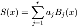 ,
,
where  are the basis spline functions (as a rule, local), and
  are numerical coefficients specifying the weight of the basis functions in forming the spline, whose physical meaning is the generalized (linear and angular) displacements of the metal ruler at the knots. The number of parameters specifying the spline equals the number of the spline's knots. There is a relationship between the segment's function parameters and the coefficients of the spline polynomial, which makes it possible to find one set of coefficients from the other, although the formulas may be fairly complex.
Converting the piecewise-polynomial representation of a spline into the basis form reduces the order of the system of linear algebraic equations used to find the unknown spline coefficients, since they are partly expressed in terms of already known parameters — the coordinates of the given points (knots) — which makes it possible to substantially reduce the computational cost by allowing the use of economical solution methods, such as the algebraic sweep method or variants of Gaussian elimination for sparse (banded) matrices with column pivoting.
Meaning of the spline's coefficients. As noted in the previous point, the meaning of a spline's parameters in the per-segment representation is determined by the type of function. In the polynomial representation, one should distinguish the case in which the coefficients have the same physical meaning as the input data, that is, the coefficients are the values of the spline at the knots. This form is called the Lagrangian form, by analogy with the Lagrange polynomial. It should be noted that the basis splines of this form equal one at the central knot and zero at all others.
The coefficients of interpolation and functional splines always contain the values of the coordinates of the given points, which follow from the interpolation conditions. Depending on the matching-derivative conditions used, they also contain the values of the corresponding derivatives at the boundaries of the spline segment (at the knot points). As a rule, when writing such conditions, the spline segment is matched at its boundaries to first or second derivatives. Matching the spline segment to first derivatives clearly reflects the physical meaning, since the first derivatives (tangents) are the angular displacements (rotations) of the metal ruler about a transverse axis. Matching a spline to second derivatives is used to simplify the form of the computational expressions, in order to reduce errors when they are copied by hand; however, in some cases, using such expressions in certain additional conditions can lead to trivial solutions.
Special splines. In a number of cases, one considers functions that lie close to the boundary between splines and ordinary functions, as well as between splines and piecewise functions. For example, these are splines consisting of two segments. They have a simplified construction but require special attention to the boundary conditions.
Special splines also include the multidimensional orthogonal normalized spline that describes a nonlinear model of an artificial neuron (the Khakimov spline model), used for modeling the dependence of a function on a set of several arguments.

Comments