
Lecture
In mathematics, analytic geometry, also known as coordinate geometry or Cartesian geometry, is the study of geometry using a coordinate system. This is different from synthetic geometry.
Analytic geometry is used in physics and engineering, as well as in aviation, rocketry, space science, spaceflight, statistics, economics, and the social sciences. It is the foundation of most modern fields of geometry, including algebraic, differential, discrete, and computational geometry.
Usually, the Cartesian coordinate system is applied to work with equations of planes, straight lines, and circles, often in two dimensions and sometimes in three. In geometry one studies the Euclidean plane (two-dimensional space) and Euclidean space. As it is taught in schools, analytic geometry can be explained more simply: it deals with defining and representing geometric figures numerically and extracting numerical information from the numerical definitions and representations of figures. The possibility of using the algebra of real numbers to obtain results about the linear continuum of geometry rests on the Cantor–Dedekind axiom.
The Greek mathematician Menaechmus solved problems and proved theorems using a method that bore a strong resemblance to the use of coordinates, and it is sometimes claimed that he introduced analytic geometry .
Apollonius of Perga, in «On Determinate Section» dealt with problems that may be called an analytic geometry of one dimension; he was concerned with finding points on a line that stood in a given ratio to others. In «Conics» Apollonius further developed a method so similar to analytic geometry that his work is sometimes considered to have anticipated that of Descartes by about 1800 years. His use of reference lines, a diameter, and a tangent is essentially no different from our modern use of a coordinate system, where distances measured along the diameter from the point of tangency are abscissas, and the segments parallel to the tangent and intercepted between the axis and the curve are ordinates. He also worked out relations between the abscissas and the corresponding ordinates that are equivalent to rhetorical equations (expressed in words) of curves. However, although Apollonius came close to developing analytic geometry, he did not succeed, because he did not take negative magnitudes into account, and in every case the coordinate system was imposed on a given curve a posteriori rather than a priori. In other words, equations were determined by curves, but curves were not determined by equations. Coordinates, variables, and equations were auxiliary notions applied to a particular geometric situation.
The 11th-century Persian mathematician Omar Khayyam saw a close relationship between geometry and algebra and was moving in the right direction when he helped narrow the gap between numerical and geometric algebra with his geometric solution of general cubic equations , but the decisive step was taken later by Descartes . Omar Khayyam is credited with laying the foundations of algebraic geometry, and his book «Treatise on Demonstrations of Problems of Algebra» (1070), which sets out the principles of analytic geometry, is part of the body of Persian mathematics that was eventually transmitted to Europe . Owing to his thoroughly geometric approach to algebraic equations, Khayyam may be regarded as a precursor of Descartes in the invention of analytic geometry
| Part of a series of articles on |
| René Descartes |
|---|
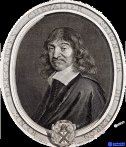 |
Analytic geometry was independently invented by René Descartes and Pierre de Fermat , although Descartes is sometimes given sole credit for it . Cartesian geometry, an alternative term used for analytic geometry, is named after Descartes.
Descartes made substantial progress with these methods in an essay titled «La Géométrie» (Geometry), one of three accompanying essays (appendices) published in 1637 together with his «Discourse on the Method of Rightly Conducting One's Reason and Seeking Truth in the Sciences», usually referred to as «Discourse on the Method». «La Geometrie», written in his native French language, and its philosophical principles laid the foundation for mathematical analysis in Europe. Initially the work was not well received, partly because of numerous gaps in the reasoning and its complicated equations. Only after it was translated into Latin and had commentary added by van Schooten in 1649 (and further work after that) did Descartes's masterpiece receive its due recognition.
Pierre de Fermat also pioneered the development of analytic geometry. Although the manuscript «Ad locos planos et solidos isagoge» (Introduction to Plane and Solid Loci) was not published during his lifetime, it circulated in Paris in 1637, shortly before the publication of Descartes's «Discourse» . Written in clear language and well received, the «Introduction» likewise laid the groundwork for analytic geometry. The key difference between the approaches of Fermat and Descartes lies in their point of view: Fermat always started from an algebraic equation and then described the geometric curve that satisfied it, whereas Descartes started from geometric curves and derived their equations as one of several properties of the curves. As a consequence of this approach, Descartes had to deal with more complicated equations and had to develop methods for working with polynomial equations of higher degree. Leonhard Euler was the first to apply the coordinate method to the systematic study of space curves and surfaces.
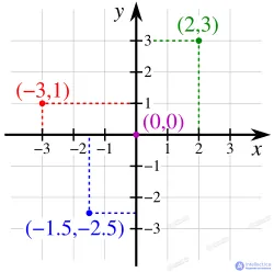
In analytic geometry, the plane is assigned a coordinate system in which every point has a pair of real-number coordinates. Similarly, Euclidean space is assigned coordinates, where each point has three coordinates. The value of the coordinates depends on the choice of the initial point, the origin. Many coordinate systems are in use, but the most common are the following:
The most common coordinate system is the Cartesian system, where each point has an x-coordinate representing its horizontal position, and a y-coordinate representing its vertical position. These are usually written as an ordered pair (x, y). This system can also be used for three-dimensional geometry, where every point in Euclidean space is represented by an ordered triple of coordinates (x, y, z).
 , passing through the points
 .
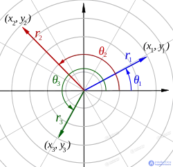
.In polar coordinates each point of the plane is represented by a distance r from the origin and an angle θ, where θ is usually measured counterclockwise from the positive x-axis. Using this notation, points are usually written as an ordered pair (r, θ). One can convert between two-dimensional Cartesian and polar coordinates using the following formulas: [ 17 ]  This system can be generalized to three-dimensional space using cylindrical or spherical coordinates. [ 17 ]
In cylindrical coordinates each point in space is represented by its height z, its radius r relative to the z-axis, and the angle θ, that its projection onto the plane xy makes with the horizontal axis.
In spherical coordinates each point in space is represented by a distance ρ from the origin, the angle θ, that its projection onto the plane xy makes with the horizontal axis, and the angle φ that it makes with the axis z. In physics, the names of these angles are often swapped.
In analytic geometry, any equation involving coordinates specifies a subset of the plane, namely the solution set of the equation, or the locus. For example, the equation y = x corresponds to the set of all points on the plane whose coordinates x and y are equal. These points form a line, and it is said that y = x is the equation of this line. In general, linear equations involving x and y, define lines, quadratic equations define conic sections, and more complicated equations describe more complicated figures.
Usually a curve on the plane corresponds to a single equation. However, this is not always the case: the trivial equation x = x defines the entire plane, while the equation x² + y² = 0 defines only a single point (0, 0). In three dimensions, a single equation usually gives a surface, and a curve must be specified as the intersection of two surfaces (see below) or as a system of parametric equations. The equation x² + y² = r² is the equation for any circle centered at the origin (0, 0 ) with radius r.
Lines in the Cartesian plane, or more generally in affine coordinates, can be described algebraically by linear equations. In the two-dimensional case, the equation for non-vertical lines is often given in slope-intercept form: where:
Just as lines in two-dimensional space are described by an equation in «point-slope» form, planes in three-dimensional space have a natural description using a point on the plane and a vector orthogonal to it (a normal vector) indicating its «tilt».
In particular, let  be the position vector of some point
  and
and  be a nonzero vector. The plane determined by this point and vector consists of those points
  with position vector
  such that the vector taken from
is perpendicular to  Recalling that two vectors are perpendicular if and only if their dot product is zero, it follows that the desired plane can be described as the set of all points such that
 (Here the dot denotes the dot product, not multiplication by a scalar.) Written out in full, this looks like: ,
 This is the point-normal form of the equation of the plane. This is simply a linear equation:
 Conversely, it is easy to show that if a, b, c and d are constants, and a, b and c are not all zero, then the graph of the equation
 is a plane having the vectoras its normal, as usual. This familiar equation for a plane is called the general form of the equation of the plane.
In three dimensions, lines cannot be described by a single linear equation, so they are often described by parametric equations:
 where:
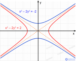
In the Cartesian coordinate system the graph of a quadratic equation in two variables always represents a conic section – although it may be degenerate, and all conic sections arise in this way. The equation will have the form: Since scaling all six constants yields the same set of zeros, conic sections can be regarded as points in five-dimensional projective space.
The conic sections described by this equation can be classified using the discriminant
 If the conic section is non-degenerate, then:
 the equation represents an ellipse;
 the equation represents a circle, which is a special case of an ellipse;
 the equation represents a parabola;
 the equation represents a hyperbola;
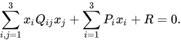
Quadric surfaces include ellipsoids (including the sphere), paraboloids, hyperboloids, cylinders, cones and planes.
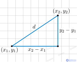
In analytic geometry, geometric notions such as distance and the measure of an angle, are defined by means of formulas. These definitions are designed to be consistent with the underlying Euclidean geometry. For example, using Cartesian coordinates in the plane, the distance between two points (x₁ , y₁) and (x₂ , y₂ ) is defined by the formula  which can be viewed as a form of the Pythagorean theorem. Similarly, the angle that a line makes with the horizontal can be defined by the formula
 where m is the slope of the line.
In three dimensions, distance is given by a generalization of the Pythagorean theorem: while the angle between two vectors is determined by the scalar product. The dot product of two Euclidean vectors A and B is defined as
  where θ is the angle between points A and B.
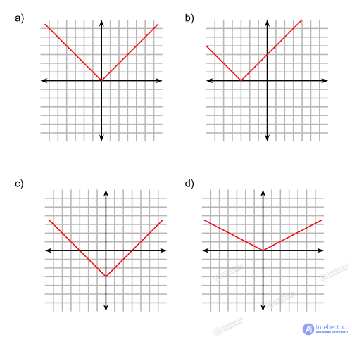
Transformations are applied to a parent function to turn it into a new function with similar characteristics.
The graph of is transformed using standard transformations as follows:
 to
to  moves the graph right
 units.
 to
to moves the graph up
 units.
 stretches the graph horizontally by a factor of
 (think of as a stretch)to
 stretches the graph vertically.to
 and changingto
 rotates the graph through angle
 .
.There are other standard transformations that are not typically studied in elementary analytic geometry, because they alter the shape of objects in ways that are not usually considered. Skewing is an example of such a transformation. For more information, see the Wikipedia article on affine transformations.
For example, the parent function has a horizontal and a vertical asymptote and lies in the first and third quadrants, and all of its transformed forms have one horizontal and one vertical asymptote and lie in either the 1st and 3rd or the 2nd and 4th quadrants. In general, if
 then it can be transformed to
  In the new transformed function,
  is a factor that stretches the function vertically if it is greater than 1, or compresses it vertically if it is less than 1, and for a negative value,the function is reflected across theaxis.The value compresses the graph horizontally if it is greater than 1, and stretches it horizontally if it is less than 1, and so on.reflects the function across theaxis when it is negative.and values introduce translations,vertical, andhorizontal. Positiveandvalues mean the function is shifted toward the positive end of its axis, while negative values mean it is shifted toward the negative end.
Transformations can be applied to any geometric equation regardless of whether the equation represents a function or not. Transformations can be considered as individual operations or in combinations.
Suppose thatis a relation in the plane. For example,
 is a relation that describes the unit circle.
For two geometric objects P and Q represented by the relations and
and the intersection is the set of all points
 that lie in both relations.
For example,might be the circle of radius 1 centered at the origin. :
:  and
and might be the circle of radius 1 centered at (1, 0).
  The intersection of these two circles is the set of points at which both equations are true. Is this true forTo find out, usingforthe equation forbecomes
 or
or which is true, solies in the relationOn the other hand, still usingforthe equation forbecomes
 or
or which is false. is not inTherefore it is not in the intersection.
The intersection ofandcan be found by solving the system of equations:


Traditional methods of finding intersections include substitution and elimination.
Substitution: Solve the first equation forin terms ofthen substitute the expression for into the second equation:

We then substitute this value in place of into the other equation and solve it for:



Next, we plug this valueinto either of the original equations and solve for:
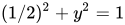


Thus we have two intersection points:
Elimination method : Add (or subtract) a multiple of one equation to the other equation so that one of the variables is eliminated. In our example, if we subtract the first equation from the second, we get  . in the first equation is subtracted fromin the second equation, leaving nothing but theterm. The variablehas been eliminated. We then solve the remaining equation for, just as in the substitution method:

Then we plug this valueinto either of the original equations and solve for:
Thus we have two intersection points:
In the case of conic sections, there can be up to 4 intersection points.
One type of intersection that is widely studied is the intersection of a geometric object with theandcoordinate axes.
The intersection of a geometric object and theaxis is called the-intercept of the object. The intersection of a geometric object and theaxis is called the-intercept of the object.
For the linethe parameterindicates the point where the line intersects theaxis. Depending on context, eitheror the point is called the-intercept.
In geometry, an axis is a line perpendicular to any given line, object, or surface.
The commonly used term for this in ordinary language is a normal (perpendicular) line, or, in engineering practice, centerline .
In geometry, a normal is an object , such as a line or vector, perpendicular to a given object. For example, in the two-dimensional case, the normal to a curve at a given point is the line perpendicular to the tangent to the curve at that point.
In the three-dimensional case, the normal to a surface at a point P is a vector perpendicular to the tangent plane to that surface at the point P. The word «normal» is also used as an adjective: a line, normal to a plane, the normal component of a force, a normal vector and so on. The concept of normality generalizes to orthogonality .
A tangent is a linear approximation of a spherical, curved, or otherwise non-straight function.
In geometry the tangent (or simply the tangent ) to a plane curve at a given point is a line , that «exactly touches» the curve at that point. Informally, it is a line passing through a pair of infinitely close points on the curve. More precisely, a line is said to be tangent to the curve y = f ( x ) at the point x = c on the curve, if the line passes through the point ( c , f ( c )) on the curve and has slope f ' ( c ) , where f ' is the derivative of the function f . The same definition applies to space curves and curves in n- dimensional Euclidean space .
Passing through the point of intersection of the tangent and the curve, called the point of tangency , the tangent line is «heading in the same direction» as the curve, and, therefore, is the best straight-line approximation to the curve at that point.
Similarly, a tangent plane to a surface at a given point is a plane that «just touches» the surface at that point. The concept of a tangent is one of the most fundamental notions in differential geometry and has been extensively generalized; see Tangent space .

Comments