Matrix Decomposition: LU Decomposition (LR), Cholesky Decomposition, and Singular Value Decomposition

Matrix decomposition is the representation of a matrix as a product of matrices possessing certain specified properties (for example, orthogonality, symmetry, diagonality). Each class of matrix decompositions has its own area of application; in particular, many efficient algorithms of computational linear algebra are based on constructing the corresponding matrix decompositions.

Decompositions for Solving Systems of Linear Algebraic Equations

LU decomposition (LU decomposition, LU factorization) is the representation of a matrix as a product of two matrices, , where is a lower triangular matrix and is an upper triangular matrix.

LU decomposition is used for solving systems of linear equations, inverting matrices, and computing the determinant. LU decomposition exists only when the matrix is invertible and all the leading (corner) principal minors of the matrix are non-singular .

This method is a variant of Gaussian elimination.

LU Decomposition

• Constraints: the matrix is square and non-singular, and all its leading principal minors are nonzero .
• Form of the decomposition: , where is a lower triangular matrix and is an upper triangular matrix. For the decomposition to be unique, it is usually additionally required that the matrix be unitriangular, i.e., a triangular matrix with diagonal entries equal to one (sometimes this unitriangularity requirement is imposed on the matrix instead) .
• Related decompositions: LDU decomposition of the form , where is a lower unitriangular matrix, is an upper unitriangular matrix, and is a diagonal matrix.
• Related decompositions: LUP decomposition of the form , where is a permutation matrix (chosen during construction of the decomposition), is a lower unitriangular matrix, is an upper triangular matrix. This is a generalization of LU decomposition to the case of arbitrary non-singular matrices.
• Existence: LUP decomposition exists for any square matrix . When the matrix reduces to the identity matrix, the LUP decomposition reduces to the LU decomposition.
• LUP and LU decompositions are used when solving the system of linear algebraic equations of dimension . The corresponding methods are variants of the matrix form of Gaussian elimination. The matrix then characterizes the combined effect of row permutations in Gaussian elimination.

Algorithm for LU Decomposition

One of the algorithms for computing the LU decomposition is given below

We will use the following notation for the matrix entries: , , , ; and the diagonal entries of the matrix , =1… .

The matrices and can be found as follows (the steps must be performed strictly in order, since later elements are computed using earlier ones):

1. Loop i from 1 to n
   1. Loop j from 1 to n
      1. u_ij=0, l_ij=0
      2. l_ii=1
2. Loop i from 1 to n
   1. Loop j from 1 to n
      1. If i<=j:
      2. If i>j:

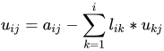
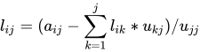
As a result we obtain the matrices and .

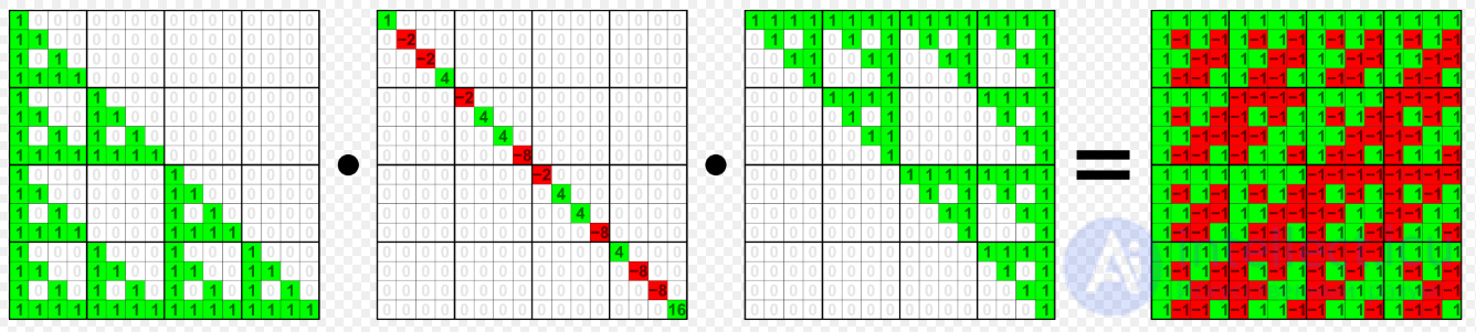fig. LDU decomposition of the Walsh matrix

Rank factorization Rank factorization

• Constraints: an arbitrary matrix of size and rank .

• Form of the decomposition: , where is a matrix of size and is a matrix of size .
• Rank factorization can be used to compute the pseudoinverse matrix, which is applied when finding the general solution of the system of linear algebraic equations .

Cholesky Decomposition

• Constraints: a symmetric positive definite matrix .
• Form of the decomposition: (or, equivalently, ), where the matrix is upper triangular (respectively, the matrix is lower triangular) .
• Related decompositions: an alternative is the modified Cholesky decomposition (LDL decomposition), which avoids taking square roots (here the matrix is a lower unitriangular matrix and is diagonal).
• The Cholesky decomposition is unique.
• The Cholesky decomposition is also applicable if the matrix is Hermitian and positive definite.
• The Cholesky decomposition is used to solve the system of linear algebraic equations , if the matrix has the corresponding properties. Compared with the LU decomposition method, this approach is guaranteed to be numerically stable and requires half as many arithmetic operations .

QR Decomposition

• Constraints: an arbitrary matrix of size .
• Form of the decomposition: , where is an orthogonal matrix of size , and is upper triangular of size .
• Related decompositions: similar QL, RQ, and LQ decompositions also exist.
• Because the matrix is orthogonal (which means its inverse coincides with its transpose ), the system is equivalent to the system with a triangular matrix, which is easy to solve.
• One way to obtain the matrix is the Gram–Schmidt process, in which case .
• Constructing the QR decomposition is the basis of the QR algorithm, one of the methods for finding the eigenvectors and eigenvalues of a matrix.
• Algorithms for solving systems of linear algebraic equations based on the QR decomposition perform almost equally well for both well-conditioned and singular systems .

Interpolative Decomposition

• Constraints: an arbitrary matrix of dimension and rank .
• Form of the decomposition: , where is a subset of indices ; the matrix consists of the corresponding columns of the original matrix; is a matrix all of whose entries do not exceed 2 in absolute value (moreover, contains an identity submatrix of dimension ). A similar decomposition can be obtained for the rows as well.

Decompositions Related to Eigenvalues or Singular Values

Spectral decomposition of a matrix

• Constraints: a diagonalizable square matrix , i.e., one having a set of distinct eigenvectors (the eigenvalues need not be distinct).
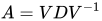• Form of the decomposition: , where is a diagonal matrix formed from the eigenvalues , and the columns of are the corresponding eigenvectors.
• Existence: a matrix of dimension always has eigenvalues (counted with multiplicity), which can be ordered (not uniquely) to form a diagonal matrix of dimension and a corresponding matrix of nonzero columns satisfying the equality . If the eigenvectors are distinct, then the matrix is invertible, which gives the desired decomposition −1 .
• The eigenvectors can always be normalized to have length 1. If is a real symmetric matrix, then is always invertible and can be normalized. In this case the matrix turns out to be orthogonal, since the eigenvectors are orthogonal to one another. Thus, the desired decomposition (which always exists in this case) can be written as .
• A necessary and sufficient condition for diagonalizability is that the geometric and algebraic multiplicities of every eigenvalue coincide. In particular, having distinct eigenvalues is a sufficient (but not necessary) condition.
• Spectral decomposition is useful for understanding the solutions of systems of linear ordinary differential equations or difference equations. For example, the difference equation with initial condition has the solution , which can also be written as 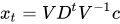(in the case that ). Computing the power of the diagonal matrix reduces to raising each element on the diagonal to the power , which is incomparably simpler than (unless, of course, the latter is already diagonal to begin with).

Jordan Normal Form Jordan Matrix

• Constraints: a square matrix .
• Form of the decomposition: , where is the Jordan matrix, and is the change-of-basis matrix.
• The Jordan normal form generalizes the diagonal form of the matrix made up of the eigenvalues, to the case where the geometric multiplicity of one or more eigenvalues is less than its algebraic multiplicity.

Schur Decomposition

• Constraints: a square matrix .
• There are two versions of the decomposition: for the case of a real matrix and for the case of a complex matrix. The latter always has a complex Schur decomposition.
• Form of the decomposition (real case): (all the matrices on both sides of the equality consist of strictly real values). In this case is an orthogonal matrix, and is quasi-triangular. The latter is called the real Schur form. The blocks on the diagonal of are either of size 1×1 (in which case they represent real eigenvalues) or 2×2 (formed by a pair of complex-conjugate eigenvalues).
• Form of the decomposition (complex case): , where is unitary, is its Hermitian conjugate, and is an upper triangular matrix, called the complex Schur form, which contains the eigenvalues on the diagonal.

QZ Decomposition Schur Decomposition, Generalized Schur Decomposition

• Constraints: square matrices and .
• There are two versions of the decomposition: complex and real.
• Form of the decomposition (complex case): , where and are unitary matrices, is the Hermitian conjugate of , and and are upper triangular matrices.
• In this decomposition, the ratio of the diagonal entries in to the corresponding entries in , , are the generalized eigenvalues, which are the solution of the generalized eigenvalue problem (where is an unknown scalar and is an unknown nonzero vector).
• Form of the decomposition (real case): , where all the matrices consist strictly of real values. are orthogonal matrices, and are quasi-triangular, consisting of blocks of size 1×1 or 2×2 (similar to the corresponding blocks in the Schur decomposition).

Singular Value Decomposition

• Constraints: an arbitrary matrix of size .
• Form of the decomposition: , where Σ is a non-negative diagonal matrix, are unitary matrices, and is the Hermitian conjugate. In the real case , where Σ, as before, is a non-negative diagonal matrix, and are orthogonal .
• The elements on the diagonal of the matrix Σ are called the singular values of the matrix and are denoted . The number of nonzero singular values of the matrix equals the rank of that matrix .
• Like spectral decomposition, singular value decomposition involves finding a basis for subspaces on whose elements the action of the operator is equivalent to multiplication by a scalar (i.e., ), but singular value decomposition is a more general method, since the matrix need not be square.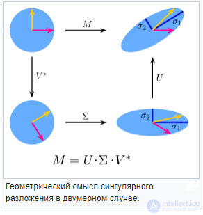

Other Decompositions

Polar Decomposition

• Constraints: a square complex matrix .
• Form of the decomposition (complex case): , where is a Hermitian matrix with non-negative leading minors, and is a unitary matrix.
• Form of the decomposition (real case): , where is a symmetric matrix with non-negative leading minors, and is an orthogonal matrix.
• For a non-singular matrix the polar decomposition is unique, while for a singular matrix only the factor is uniquely determined.
• In the complex case, the polar decomposition of a matrix is analogous to representing an arbitrary complex number in the form .

Frobenius Normal Form

• Constraints: a square matrix .
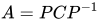• Form of the decomposition:, where is a block-diagonal matrix composed of the companion matrices of monic polynomials such that is a multiple of . is the transition matrix.

See Also

• Matrix splitting
• Non-negative matrix factorization
• Principal component analysis