
Lecture
An eigenvector is a concept in linear algebra, defined for an arbitrary linear operator as a nonzero vector to which applying the operator gives a collinear vector — the same vector multiplied by some scalar value (which may be equal to 0). The scalar by which the eigenvector is multiplied under the action of the operator is called the eigenvalue (or characteristic value) of the linear operator corresponding to this eigenvector. One representation of a linear operator is a square matrix, so eigenvectors and eigenvalues are often defined in the context of using such matrices .
The concepts of eigenvector and eigenvalue are among the key notions in linear algebra, and many constructions are built upon them. This is because many relations involving linear operators are considerably simplified in a coordinate system built on a basis of the operator's eigenvectors. The set of eigenvalues of a linear operator (the spectrum of the operator) characterizes important properties of the operator independently of any particular coordinate system. For these reasons, eigenvectors are of significant practical importance. For example, eigenvectors are frequently encountered in mechanics, quantum theory, and so on. In particular, the spin projection operator onto an arbitrary axis has two eigenvalues and the corresponding eigenvectors.
The concept of a linear vector space is not limited to «purely geometric» vectors and generalizes to various sets of objects, such as function spaces (on which linear differential and integral operators act). For spaces and operators of this kind, one speaks of the eigenfunctions of the operators.
The set of all eigenvectors of a linear operator corresponding to a given eigenvalue, together with the zero vector, is called the eigenspace of that operator.
Finding optimal algorithms for computing the eigenvalues of a given linear operator is one of the important problems in computational mathematics.
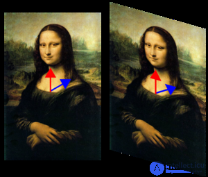
Another transformation of the Mona Lisa. The blue vector changes direction, while the red one does not. Therefore, the red vector is an eigenvector, while the blue one is not. Since the red vector was neither stretched nor compressed, its eigenvalue, as in the picture above, equals one. Any vector collinear with the red one is also an eigenvector.
An eigenvector of a linear transformation  , where L
 is a linear space over a field K
 , is a nonzero vector
  such that for some
  the relation
  holds.
An eigenvalue (characteristic value) of a linear transformation A is a number λ∈K for which an eigenvector exists, that is, the equation Ax=λx has a nonzero solution .
Simply put, an eigenvector is any nonzero vector x that the operator A maps to a vector λx collinear with it, and the corresponding scalar λ is called the eigenvalue of the operator.
An eigenspace (or characteristic subspace) of a linear transformation A for a given eigenvalue λ∈K (or corresponding to that eigenvalue) is the set of all eigenvectors corresponding to that eigenvalue, together with the zero vector. Let us denote the eigenspace corresponding to the eigenvalue λ
 by Eλ
by Eλ , and the identity operator by I
 . By definition, the eigenspace is the kernel of the operator A−λ⋅I,
 that is, the set of vectors mapped by this operator to the zero vector:
 .
.
A root vector of a linear transformation A for a given eigenvalue λ∈K is a nonzero vector x∈L such that for some natural number m the following holds:
 .
.
If m is the smallest of such natural numbers (that is,  ), then m is called the height of the root vector x
 .
.
The root subspace of a linear transformation A for a given eigenvalue is the set of all root vectors corresponding to that eigenvalue, if this set is supplemented with the zero vector. Let us denote the root subspace corresponding to the eigenvalue λ by  . By definition:
 .
.

The blue color marks the eigenvector. Unlike the red one, it did not change direction under the deformation (transformation), so it is an eigenvector of this transformation, corresponding to some eigenvalue λ (here it equals one, since the vector did not change its length). Any vector parallel to the blue vector will also be an eigenvector corresponding to the same eigenvalue. The set of all such vectors (together with the zero vector) forms the eigenspace
Eigenvalues are usually introduced in the context of linear algebra, but historically they arose in the study of quadratic forms and differential equations.
In the 18th century, Euler, studying the rotational motion of an absolutely rigid body, discovered the significance of the principal axes, and Lagrange showed that the principal axes correspond to the eigenvectors of the inertia matrix. In the early 19th century, Cauchy used the work of Euler and Lagrange to classify second-order surfaces and generalized the results to higher orders. Cauchy also introduced the term «characteristic root» (French: racine caractéristique) for the eigenvalue. This term has survived in the context of the characteristic polynomial of a matrix.
In the early 20th century, Hilbert studied the eigenvalues of integral operators, treating the latter as infinite-dimensional matrices . In 1904, to denote eigenvalues and eigenvectors, Hilbert began using the terms eigenvalues and eigenvectors, based on the German word eigen (own/characteristic). These terms subsequently passed into English as well, replacing the previously used terms «proper value» and «proper vector».
The subspace  is called an invariant subspace of a linear transformation A (an A-invariant subspace) if:
 .
.
The eigenspaces , the root subspaces Vλ, and the subspaces  of a linear operator A are A-invariant.
Eigenvectors are root vectors (of height 1): λ ;
;
Root vectors need not be eigenvectors: for example, for a transformation of a two-dimensional space given by the matrix:
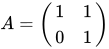
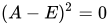 , and all vectors are root vectors corresponding to the eigenvalue 1, but A has a single eigenvector (up to multiplication by a number).
For different eigenvalues, the root (and hence eigen-) subspaces have a trivial (zero) intersection:
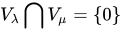 if
if  .
.
The Courant—Fischer theorem gives a method for finding the eigenvalues of self-adjoint operators and finding the singular values of a normal operator.
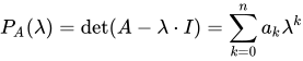
Having chosen a basis in an n -dimensional linear space L, one can associate a square n×n matrix with the linear transformation and define its characteristic polynomial:
 .
.
The characteristic polynomial does not depend on the basis in L. Its coefficients are invariants of the operator A. In particular,  , an−1=trA
 do not depend on the choice of basis.
The eigenvalues, and only they, are the roots of the characteristic polynomial of the matrix. The number of distinct eigenvalues cannot exceed the size of the matrix. If the eigenvectors of the operator are chosen as the basis vectors, then the matrix A becomes diagonal in that basis, with the eigenvalues of the operator on the diagonal. Note, however, that not every matrix admits a basis of eigenvectors (the general structure is described by the Jordan normal form). For a positive-definite symmetric matrix A, the procedure for finding the eigenvalues and eigenvectors is nothing other than finding the directions and lengths of the semi-axes of the corresponding ellipse.
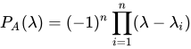
If the number field is algebraically closed (for example, the field of complex numbers), then the characteristic polynomial factors into a product of n linear factors:
 ,
,
where  are the eigenvalues; some of the λi
 may be equal. The multiplicity of an eigenvalue is the number of factors equal to
  in the factorization of the characteristic polynomial into linear factors (also called the algebraic multiplicity of the eigenvalue).
The dimension of the root space  equals the multiplicity of the eigenvalue.
The vector space L decomposes into a direct sum of root subspaces (by the theorem on the Jordan form):

where the summation is over all λi — the eigenvalues of A.
The geometric multiplicity of an eigenvalue λi is the dimension of the corresponding eigenspace  ; the geometric multiplicity of an eigenvalue does not exceed its (algebraic) multiplicity, since
All root vectors of a normal operator are eigenvectors. Eigenvectors of a normal operator A corresponding to different eigenvalues are orthogonal, that is, if Ax=λx, Ay=μy and λ≠μ, then (x,y)=0 (this is not true for an arbitrary operator).
All eigenvalues of a self-adjoint operator are real, those of an anti-Hermitian operator are imaginary, and all eigenvalues of a unitary operator lie on the unit circle |λ|=1 .
.
In the finite-dimensional case, the sum of the dimensions of the eigenspaces of a normal operator  corresponding to all eigenvalues equals the dimension of the matrix, and the vector space decomposes into an orthogonal sum of eigenspaces:
 ,
,
where the summation is over all λi — the eigenvalues of A, and are mutually orthogonal for different λi. This property is characteristic of a normal operator over C in the finite-dimensional case: an operator is normal if and only if its matrix has diagonal form in some orthonormal basis.
A square real n×n matrix  is called positive if all its elements are positive:
  .
.
Perron's theorem (a special case of the Perron—Frobenius theorem): A positive square matrix A has a positive eigenvalue r, which has algebraic multiplicity 1 and strictly exceeds the absolute value of any other eigenvalue of this matrix. The eigenvalue r corresponds to an eigenvector  , all of whose coordinates are strictly positive. The vector is the only eigenvector of A (up to multiplication by a number) having non-negative coordinates.
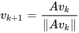
The eigenvector can be computed by direct iteration: an arbitrary initial vector  with positive coordinates is chosen, and each subsequent element is given by the recurrence formula:
 ,
,
yielding a sequence  , converging to the normalized eigenvector
  .
.
Another application of the direct iteration method is finding the eigenvectors of positive-definite symmetric operators.
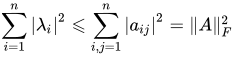
Schur's inequality: for the eigenvalues  of the matrix
  :
:
 ,
,
with equality holding if and only if A is a normal matrix.
For the eigenvalues λ1,...,λn of the matrix A=B+iC, where the matrices B,C are Hermitian, the following holds:
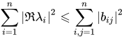 and
and 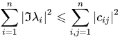 .
.
For Hermitian matrices  and
and  , their eigenvalues, arranged in increasing order:
  give:
give:  for
for  and γi
 for i≤j
 .
.
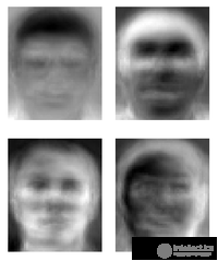
Eigenfaces as examples of eigenvectors
In image processing, processed face images can be treated as vectors whose components are the brightness of each pixel. The dimension of this vector space is the number of pixels. The eigenvectors of the covariance matrix associated with a large set of normalized face images are called eigenfaces; this is an example of principal component analysis. They are very useful for expressing any face image as a linear combination of some of them. In the branch of biometrics dealing with face recognition, eigenfaces provide a means of applying data compression to faces for identification purposes. Research has also been carried out on eigen-vision systems for determining hand gestures.
Similarly, eigenvoices represent a general direction of variability in the human pronunciation of a specific utterance, for example, a word in a language. A new vocal pronunciation of a word can be constructed based on a linear combination of such eigenvoices. These concepts have proven useful in automatic speech recognition systems for speaker adaptation.

Comments