
Lecture
Second-order curves and surfaces are an important class of geometric objects described by second-degree equations in their variables. They play a key role in analytic geometry and are widely used in physics, engineering, and other fields.
A second-order curve is the locus of points in a plane whose rectangular coordinates satisfy an equation of the form
a11x2+2a12xy+a22y2+2a13x+2a23y+a33=0,
in which at least one of the coefficients a11, a12, a22 is nonzero. Thus a second-order curve is a special case of an algebraic curve.
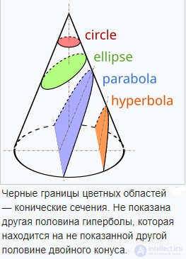
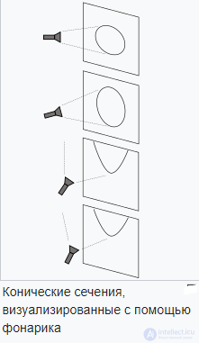
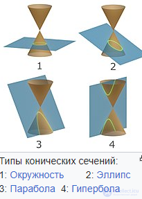
Second-order curves were first studied by Menaechmus, a student of Eudoxus. His approach was as follows: if two intersecting lines are rotated about the bisector of the angle they form, a conical surface is obtained. If this surface is then cut by a plane, the cross-section yields various geometric figures, namely an ellipse, a circle, a parabola, a hyperbola, and several degenerate figures (see below).
However, this knowledge found practical application only in the 17th century, when it became known that planets move along elliptical trajectories and a cannonball follows a parabolic path. Later still it became known that if a body is given the first cosmic velocity, it will move in a circle around the Earth; as this velocity increases — along an ellipse; upon reaching the second cosmic velocity — along a parabola; and at a velocity greater than the second cosmic velocity — along a hyperbola.
The type of curve depends on four invariants:
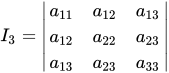 (also denoted Δ
 )
) (also denoted D
 )
) (also denoted I
 )
)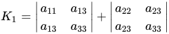 (also denoted B
 )
)The expression «invariant of a curve», sometimes encountered, is imprecise. If the equation is multiplied by a nonzero number k, the resulting equation defines the same curve. In doing so the values of the invariants change.  and so on.
| Curve | Equation | Invariants | |||
|---|---|---|---|---|---|
| Ellipse | 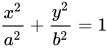 |
 |
 |
 |
|
| Point (pair of imaginary intersecting lines) | 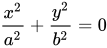 |
 |
|||
| Imaginary ellipse | 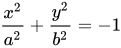 |
 |
|||
| Hyperbola | 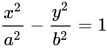 |
 |
 |
||
| Pair of intersecting lines | 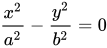 |
|
|||
| Parabola |  |
 |
|
||
| Pair of parallel lines |  |
|
 |
||
| Line |  |
 |
|||
| Pair of imaginary parallel lines |  |
 |
A second-order curve is called non-degenerate if Δ≠0. The following cases can arise:

 and Δ⋅I<0
 ;
;
 or a11=a22,a12=0;
 and Δ⋅I>0;


A second-order curve is called degenerate if Δ=0 . The following cases can arise:


Many important properties of second-order curves can be studied using the characteristic quadratic form corresponding to the equation of the curve

Thus, for example, a non-degenerate curve (Δ≠0) turns out to be a real ellipse, an imaginary ellipse, a hyperbola, or a parabola depending on whether F0(x,y)
 is a positive-definite, negative-definite, indefinite, or semi-definite quadratic form, which is determined from the roots of the characteristic equation:
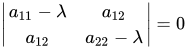
or

The roots of this equation are the eigenvalues of the real symmetric matrix
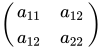
and, as a consequence, are always real.
The diameter of a second-order curve is the locus of midpoints of parallel chords of that curve. The diameter obtained in this way is called conjugate to these chords, or to their direction. The diameter conjugate to chords making an angle θ with the positive direction of the Ox axis is given by the equation:

If the condition D≠0 holds, then all diameters of the curve intersect at a single point — the center — and the curve itself is called central. Otherwise (D=0), all diameters of the curve are either parallel or coincide.
The coordinates of the center (x0,y0) are determined by the system of equations:
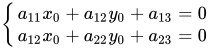
Solving this system for  and
and  we obtain:
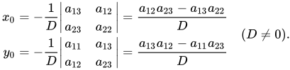
If the curve is central, translating the origin to its center reduces the equation to the form

where are the coordinates relative to the new system.
The principal axis of a second-order curve is its diameter that is perpendicular to the chords conjugate to it. This diameter is an axis of symmetry of the curve. Every central curve (D≠0) either has two mutually perpendicular axes, or all of its diameters are principal axes. In the latter case the curve is a circle. Non-central curves (D=0)
 have only one principal axis. The points where the principal axis meets the curve itself are called its vertices.
The direction cosines of the normals to the principal axes satisfy the equations

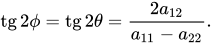
where λ is a nonzero root of the characteristic equation. The directions of the principal axes and of the chords conjugate to them are called the principal directions of the curve. The angle between the positive direction of the Ox axis and each of the two principal directions is given by the formula
Of all types of second-order curves, only the circle has indeterminate principal directions.
The general equation of the curve can be written in matrix form
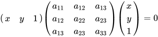 or x
or x
By introducing a new coordinate system, the equations of second-order curves can be reduced to the standard canonical form (see the table above). The parameters of the canonical equations are expressed quite simply in terms of the invariants Δ,D,I of the original curve equation and the roots of the characteristic equation λ1⩾λ2
 (see the section «Characteristic quadratic form and characteristic equation» above).
Remark. When passing to the canonical form, it may be necessary to multiply the equation by a nonzero number. Therefore the numerical values of the invariants of the canonical equation may differ from the values of the invariants of the original equation. The signs of the quantities Δ⋅I and D remain unchanged.
For a central curve in canonical form, its center (x0,y0) lies at the origin.
The canonical equation of any non-degenerate second-order curve can, by means of a suitable transformation of the origin, be reduced to the form

In this case the curve passes through the origin of the new coordinate system, and the Ox axis is an axis of symmetry of the curve. This equation expresses the fact that a non-degenerate second-order curve is the locus of points for which the ratio of the distances ε⩾0 (eccentricity) from a given point (the focus) and from a given line (the directrix) is constant. Moreover, at ε=0
 the curve is a circle, at ε<1
 — an ellipse, at ε=1
 — a parabola, at ε>1
 — a hyperbola.
The equation of the directrix of the curve is expressed by x=−pε(1+ε),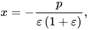 and the coordinates of the focus by x=p1+ε,y=0.
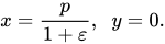 The directrix is perpendicular to the axis of symmetry that passes through the focus and the vertex of the curve (the focal axis). The distance between the focus and the directrix equals pε.
If the second-order curve is central (an ellipse or a hyperbola), then the line
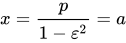
is an axis of symmetry, and consequently the curve has two foci and two directrices.
The parameter  is called the focal parameter and equals half the length of the chord passing through the focus and perpendicular to the focal axis (the focal chord).
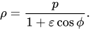
If the pole of the polar coordinate system (ρ,ϕ) is taken to be the focus of a non-degenerate second-order curve, and the polar axis to be its axis of symmetry, then in the polar coordinates ρ
 , ϕ
, ϕ the equation of the curve takes the form
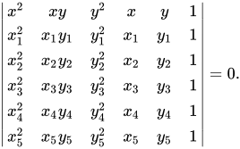
A second-order curve is completely determined by five of its points, provided that no four of them lie on the same line. The equation of the curve passing through the points (x1,y1), (x2,y2), (x3,y3), (x4,y4) and (x5,y5):
.
A curve given by five points degenerates if and only if three of the given points lie on the same line.
The equation of the tangent to a second-order curve f(x,y) at its point (x1,y1)
 has the form:

The equation of the normal to a second-order curve at the point (x1,y1) has the form

The equation

besides the tangent, defines a line called the polar of the point (x1,y1) with respect to the second-order curve, regardless of whether this point lies on the curve or not. The point (x1,y1) is then called the pole of this line. The polar of a point of the curve is its tangent at that point.
Theorems about poles and polars:
 intersects the polar at a point Q,
 and the second-order curve at points R1
 and R2,
 then the points P
 and Q
and Q harmonically divide the segment R1R2,
 that is, the following condition holds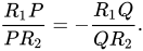
From these statements, in particular, it follows that:
Second-order surfaces
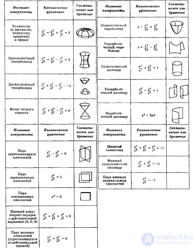
Second-order curves and surfaces are used in various fields:
Conic sections are important in astronomy: the orbits of two massive objects that interact according to Newton's law of universal gravitation are conic sections if their common center of mass is considered to be at rest. If they are bound together, they will both trace out ellipses; if they are unbound, they will both follow parabolas or hyperbolas. See the two-body problem.
The reflective properties of conic sections are used in the design of searchlights, radio telescopes, and some optical telescopes. A searchlight uses a parabolic mirror as a reflector with a bulb at the focus; a similar design is used for a parabolic microphone. The 4.2-meter Herschel optical telescope on the island of La Palma, in the Canary Islands, uses a primary parabolic mirror to reflect light toward a secondary hyperbolic mirror, which reflects it back to a focus behind the primary mirror.
These objects play an important role in mathematical modeling and real-world applications owing to their unique geometric properties.

Comments