Covariance and Contravariance (Mathematics)

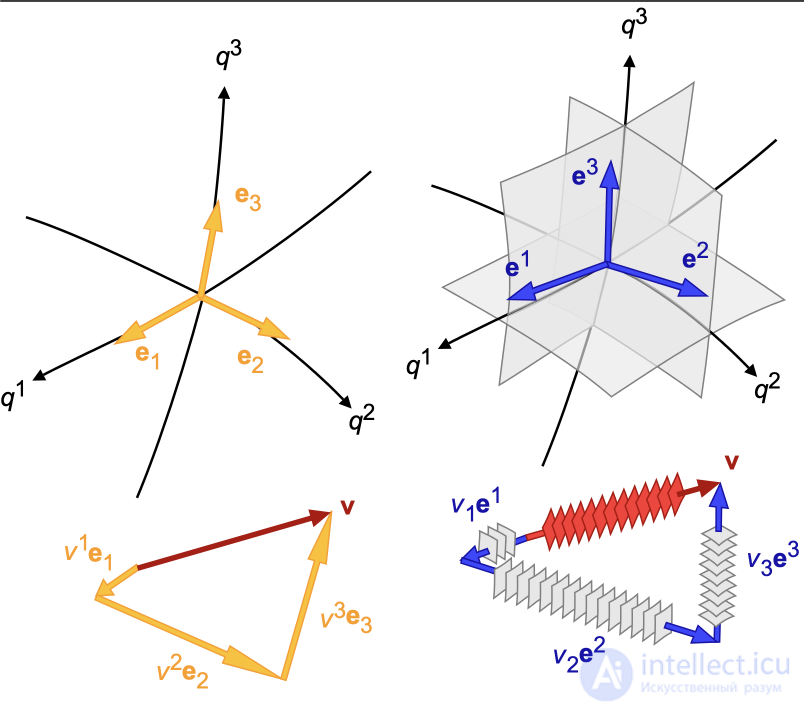
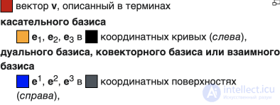
Let $$ be some finite-dimensional vector space, with some basis defined in it. An arbitrary vector $x$ can be represented as a linear combination of the basis vectors: ${\mathrm{<br>\; i}}_{}$. To simplify the notation (and for reasons that will become clear below), let us denote the coordinates with an upper index and adopt Einstein's convention: whenever the same index appears at different levels in an expression, summation over it is implied. Thus we can write:i. Let us define a new basis by means of the transformation matrix $S$. For the same reasons, let us introduce lower and upper indices (so as not to have to write summation signs) — $S_i^j$. Then ${}_{}^{}$
(summation over the index j is implied). Denoting the inverse matrix $$
, we can write: ${}_{}$
. Substituting this formula into the coordinate representation of the vector x, we obtain: $$. Thus the coordinates of the vector in the new basis turn out to equal ${}^{}$
j, that is, they transform "oppositely" (inversely) to the change of basis. For this reason such vectors are called contravariant — changing opposite to the basis. Contravariant vectors are ordinary vectors. In coordinate representation, contravariant vectors are usually written as a "column vector". An upper, or contravariant, index is used to identify contravariant vectors.

The space of all linear functionals mapping vectors to numbers is called the dual space ${}^{}$. It is also a vector space of the same dimension as the original space. A basis can likewise be defined in this space. Let us denote the elements of the basis of the dual space with an upper index $g^i$. Any functional can be represented in this basis through coordinates, which we will denote with lower indices. Then, applying Einstein's convention, we can write: $$
, that is, any linear functional can simply be written as a set of numbers $f_i$, just like an ordinary vector (except that the index is placed as a subscript).

Let us choose a basis in the dual space such that $g^i\left(x\right)=x^i$, that is, these functionals return the $i$-th coordinate of the vector (the projection onto the basis vector $e_i$). Such a basis is called dual (to the basis of the original space). When the basis of the original space is changed, this condition must be preserved, that is,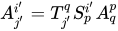 $A_{j^{\prime }}^{i^{\prime }}=T_{j^{\prime }}^q{S}_p^{i^{\prime }}{A}_q^p$

In general, one must understand that the object itself does not depend on its representation in a basis. All the transformations are merely representations of one and the same object (a tensor).

If a linear space is equipped with a scalar product $g$ — a bilinear form (or, in tensor terminology, a twice-covariant tensor) possessing the properties of symmetry and non-degeneracy — then such (finite-dimensional) spaces are called Euclidean (provided the corresponding quadratic form $g(x,x)$ is positive definite) or pseudo-Euclidean (with no restriction on the sign of the quadratic form). The tensor corresponding to this bilinear form is called the metric tensor. The components of this tensor in a given basis are 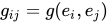${}_{}$. If this basis is orthonormal (such a basis always exists in a (pseudo-)Euclidean space), then the matrix of components is diagonal. On the diagonal, in the case of a Euclidean space, are ones (the identity matrix). In the case of a pseudo-Euclidean space, besides ones, the diagonal also contains "minus-ones". In the general case, however, the bases may be non-orthogonal, so the metric tensor may also be represented by a non-diagonal matrix (nevertheless, in a "flat" space there always exists a change of basis that brings it to diagonal form).

With the help of the metric tensor, the scalar product can be written as 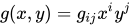$g(x,y)=g_{ij}{x}^i{y}^j$. In spaces with a scalar product there is a canonical isomorphism between the space $V$ and the dual space $V^{\ast }$, that is, each vector corresponds to a covector and vice versa. This correspondence is established precisely by means of the scalar product, or, in tensor notation, by means of the metric tensor. Namely, we can write $x_i=g_{ij}{x}^j$. This operation is called lowering or dropping an index. The inverse correspondence is established by means of the contravariant metric tensor $x^j=g^{ij}{x}_i$. This operation is called raising or lifting an index. It is easy to show that the matrices of the covariant and contravariant metric tensors are mutually inverse, that is, $g_{ik}{g}^{kj}={\delta }_i^j$. The scalar product can be expressed both in contravariant and in covariant vectors: <span about="#mwt69" class="mwe-math-element mwe-math-element-inline" data-mw="{" id="mwlg" j="x_iy^i=x^iy_i=g^{ij}x_iy_j" }}"""="" style="white-space: nowrap;" typeof="mw:Extension/math">$g(x,y)=g_{ij}{x}^i{y}^j=x_i{y}^i=x^i{y}_i=g^{ij}{x}_i{y}_j$.

In the case of an orthonormal basis in a Euclidean space, the metric tensor is the identity matrix, so a covariant vector in coordinate notation coincides with the corresponding contravariant one. In this case, therefore, dividing vectors into contravariant and covariant is not necessary. However, as soon as the basis becomes non-orthogonal and/or the space becomes pseudo-Euclidean, this distinction becomes significant. In a pseudo-Euclidean space, in an orthogonal basis, covectors differ from the corresponding ordinary vector in the signs of some of their coordinates. In such a case, the system of vectors and covectors makes it possible to write the formula for the squared length of a vector in the same way as in the Euclidean case $x_i{x}^i$. In the case of non-orthogonal (oblique) bases in Euclidean (pseudo-Euclidean) spaces, the metric tensor that converts contravariant vectors into covariant ones is not diagonal. Here, too, the length of a vector is written in the same way as in a Euclidean space, using contravariant and covariant vectors. All these cases have one thing in common — the metric tensor (in a given basis) has the same matrix for all points (vectors) of the space.

In spaces with a metric tensor, a "covariant vector" and a "contravariant vector" are in fact different representations (records in the form of a set of numbers) of one and the same geometric object — an ordinary vector or covector. That is, the same vector can be written as covariant (that is, as a set of covariant coordinates) and as contravariant (that is, as a set of contravariant coordinates). The same can be said of a covector. Converting one representation into the other is done simply by contraction with the metric tensor. In substance, vectors and covectors are distinguished only by which of the representations is natural for them. The contravariant representation is natural for an ordinary vector. For a covariant vector, what is natural is contraction with ordinary vectors without involving the metric. An example of a covariant vector is the gradient of a scalar function 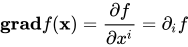$$. Its contraction with a contravariant (ordinary) vector $$ gives an invariant — the differential of the function $$. Thus, if we take $$ to be ordinary vectors of the space, then the gradient must be a covector, so that no metric tensor is needed when contracting. At the same time, the vectors $$
themselves require the use of the metric tensor $$ when contracted with vectors of the same kind.

If we are dealing with ordinary physical space, a simple criterion for the covariance or contravariance of a vector is how its natural representation contracts with the set of coordinates of a spatial displacement $d{x}^i$, which is a model contravariant vector. Those that contract with $d{x}^i$ by simple summation, without involving the metric, are covariant vectors, while those that require the metric are contravariant vectors. If, however, the space and the coordinates are so abstract that there is no way to distinguish the primary basis from the dual one other than by an arbitrary, conventional choice, then the substantive distinction between covariant and contravariant vectors disappears, or likewise becomes purely conventional.

A covariant vector, especially in the physical literature, is often taken to mean the expansion of any vector (that is, of a vector or covector, a vector of the tangent or cotangent space) in the dual basis. This then refers to the set of covariant coordinates of any object; usually, however, each type of object is written in the basis natural to it, which corresponds to the primary definition.

In the case of curvilinear coordinates or curved spaces, the new coordinates are, generally speaking, nonlinear functions of the old coordinates: $x^{\prime i}=x^{\prime i}(x^1,x^2,...,x^n)$. For infinitesimal changes of the old coordinates $d{x}^j$, the changes in the new coordinates can be defined via the Jacobian matrix of the above functions:

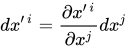
Any vector $v$ that transforms in the same way as $d{x}^i$, that is

$v^{\prime i}=\frac{\partial x^{\prime i}}{\partial x^j}{v}^j$

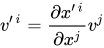
is called a contravariant vector.

For some scalar function of the coordinates $$f(x) consider its gradient . When passing to other coordinates, we have:

$\frac{\partial f\left(x\right)}{\partial x^{\prime i}}=\frac{\partial f\left(x\right)}{\partial x^j}\frac{\partial x^j}{\partial x^{\prime i}}$

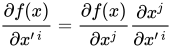
Any vector $u$ that transforms in the same way as the gradient, that is

${A^{\prime }}_{ij}=\frac{\partial x^q}{\partial x^{\prime i}}\frac{\partial x^p}{\partial x^{\prime j}}{A}_{pq}$

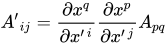
And for a tensor that is once contravariant and once covariant, the transformation law has the form:

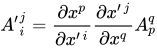
Usually, to indicate that the components of a tensor have been transformed to a new, primed basis, the prime is placed on the corresponding indices of the tensor rather than on its letter symbol; in that case the above formulas are written as follows