The Concept of a Matrix as a Mathematical Object, Operations on Matrices, and Applications

A matrix is a mathematical object represented as a rectangular array of elements of a ring or field (for example, integers, real, or complex numbers), consisting of a set of rows and columns at whose intersections its elements are located. The number of rows and columns determines the size of the matrix. Although triangular matrices, for example, were considered historically, nowadays the term is used exclusively for matrices of rectangular form, since these are the most convenient and general.

Matrices are widely used in mathematics for the compact notation of systems of linear algebraic or differential equations. In this case, the number of rows of the matrix corresponds to the number of equations, and the number of columns to the number of unknowns. As a result, solving systems of linear equations reduces to operations on matrices.

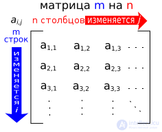
Matrix structure

The following algebraic operations are defined for a matrix:

• addition of matrices of the same size[⇨];
• multiplication of matrices of compatible size (a matrix with columns can be multiplied on the right by a matrix with rows)[⇨];
• including multiplication of a vector by a matrix (according to the usual rule of matrix multiplication; in this sense a vector is a special case of a matrix)[⇨];
• multiplication of a matrix by an element of the underlying ring or field (that is, a scalar)[⇨].

With respect to addition, matrices form an abelian group; if multiplication by a scalar is also considered, matrices form a module over the corresponding ring (a vector space over a field). The set of square matrices is closed under matrix multiplication, so square matrices of the same size form an associative ring with identity under matrix addition and matrix multiplication.

It can be proved that a unique square matrix of order n can be associated with every linear operator acting in an n-dimensional linear space; and conversely, a unique linear operator acting in that space can be associated with every square matrix of order n. The properties of the matrix correspond to the properties of the linear operator. In particular, the eigenvalues of the matrix are the eigenvalues of the operator corresponding to the respective eigenvectors.

The same can be said about the representation of bilinear (quadratic) forms by matrices.

Mathematics considers many different types and kinds of matrices. These include, for example, identity, symmetric, skew-symmetric, upper triangular (lower triangular), and other such matrices.

Normal forms — that is, the canonical form to which a matrix can be reduced by a change of coordinates — hold special significance in matrix theory. The theory of Jordan normal forms is the most important (in the theoretical sense) and the most thoroughly developed. In practice, however, normal forms that possess additional properties, such as stability, are used.

History[ | ]

Matrices were first mentioned as far back as ancient China, where they were called a «magic square». The main application of matrices was the solution of linear equations. Magic squares also became known somewhat later to Arab mathematicians, and it was around that time that the principle of matrix addition appeared. After the theory of determinants developed at the end of the 17th century, Gabriel Cramer began developing his own theory in the 18th century and published «Cramer's rule» in 1751. The «Gaussian elimination» method appeared at around the same time. The theory of matrices came into being in the mid-19th century in the works of William Hamilton and Arthur Cayley. Fundamental results in matrix theory are due to Weierstrass, Jordan, and Frobenius. The term «matrix» was introduced by James Sylvester in 1850.

Introduction[ | ]

Matrices arise naturally when solving systems of linear equations, as well as when considering linear transformations.

Systems of Linear Equations

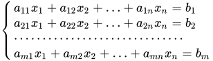
Consider a system of linear equations of the form:

.

This system consists of linear equations in unknowns. It can be written as the following matrix equation:

,

where

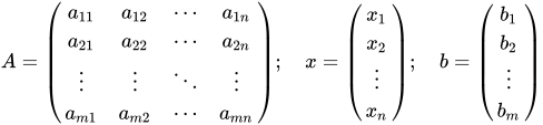
The matrix is the matrix of coefficients of the system of linear equations, the column vector is the vector of unknowns, and the column vector is some given vector.

For the system to have a solution (at least one), it is necessary and sufficient that the vector be a linear combination of the columns of , and then the vector is the vector containing the coefficients of the expansion of the vector in terms of the columns of the matrix.

In terms of matrices, the solvability condition for a system of linear equations is formulated as the Kronecker-Capelli theorem:

the rank of the matrix equals the rank of the augmented matrix ,

formed from the columns of and the column .

Important special case. If the number of equations equals the number of unknowns (, i.e., the matrix is square), then the condition for a unique solution is equivalent to the condition that the matrix is invertible.

(Remark. Solvability of the system does not by itself imply that the matrix is non-singular. Example: .)

In particular, if the matrix is invertible, then the solution of the system can be written (and, if has been computed, also found) in the form

.

This leads to an algorithm for computing the values of the unknowns using Cramer's rule.

Linear Transformations[ | ]

Linear mapping

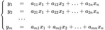
Consider a linear transformation acting from an -dimensional vector space to an -dimensional vector space , having the following form:

.

In matrix form, this transformation is an equation of the form:

.

The matrix is the coefficient matrix of the linear transformation.

If we consider the action of the linear transformation on vectors of the form

,

forming a basis of the space , then is the j-th column of the matrix .

Thus, the matrix completely describes the linear transformation , and is therefore called the matrix of the linear transformation.

Definitions[ | ]

Rectangular Matrix[ | ]

Let there be two finite sets:

• row indices: ;

• column indices: , where and are natural numbers.

Let us call a matrix of size (read as by ) ( - rows, - columns) with elements from some ring or field a mapping of the form . The matrix is written as

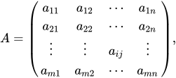
where the matrix element is located at the intersection of the -th row and the -th column.

• -th row of the matrix
• -th column of the matrix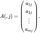

The total number of elements of the matrix is .

Accordingly,

• each row of the matrix can be interpreted as a vector in the -dimensional coordinate space ;
• each column of the matrix — as a vector in the -dimensional coordinate space .

The matrix itself is naturally interpreted as a vector in the space , having dimension . This makes it possible to introduce componentwise addition of matrices and multiplication of a matrix by a number (see below); as for matrix multiplication, it relies essentially on the rectangular structure of the matrix.

Square Matrix[ | ]

If a matrix has a number of rows equal to the number of columns , then the matrix is called square, and the number is called the size of the square matrix, or its order.

Row Vector and Column Vector[ | ]

Matrices of size and are elements of the spaces and respectively:

• a matrix of size is called a column vector and has the special notation: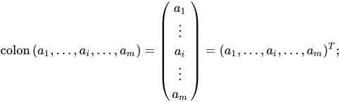

• a matrix of size is called a row vector and has the special notation:

Elementary Transformations of Matrices

The following transformations of the rows of a matrix are called elementary transformations:

1. Multiplying a row by a number other than zero,
2. Adding one row to another row,
3. Swapping two rows.

Elementary transformations of the columns of a matrix are defined analogously.

Rank of a Matrix[ | ]

Rank of a matrix

The rows and columns of a matrix are elements of the corresponding vector spaces:

• the columns of the matrix are elements of a space of dimension ;
• the rows of the matrix are elements of a space of dimension .

The rank of a matrix is the number of linearly independent columns of the matrix (the column rank of the matrix) or the number of linearly independent rows of the matrix (the row rank of the matrix). Equivalent to this definition is the definition of the rank of a matrix as the order of the largest nonzero minor of the matrix.

Elementary transformations do not change the rank of a matrix.

Notation[ | ]

A matrix is usually denoted by a capital letter of the Latin alphabet: let

then is a matrix that is interpreted as a rectangular array of elements of the field of the form , where

• the first index denotes the row index: ;
• the second index denotes the column index: ;

thus, is the element of the matrix located at the intersection of the -th row and the -th column. Accordingly, the following compact notation is adopted for a matrix of size :

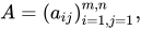
or simply

if it is only necessary to indicate the notation for the elements of the matrix.

Sometimes, instead of , one writes , in order to separate the indices from one another and avoid confusion with the product of two numbers.

If a detailed representation of the matrix as a table is required, the following notation is used

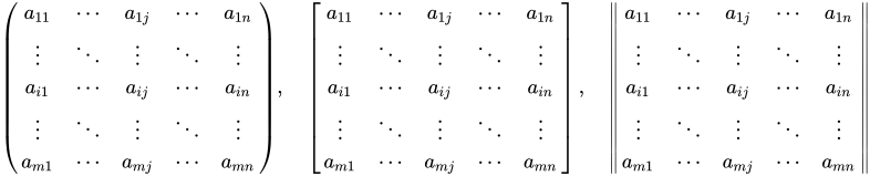
One can encounter notation with round brackets «(…)», as well as notation with square brackets «[…]». Less often, one may encounter notation with double straight lines «||…||»).

Since a matrix consists of rows and columns, the following notations are used for them:

is the -th row of the matrix ,

and

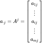is the -th column of the matrix .

Thus, a matrix has a dual representation — by columns:

and by rows:

.

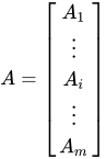This representation makes it possible to formulate properties of matrices in terms of rows or in terms of columns.

Transposed Matrix

For every matrix 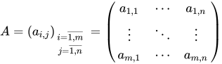of size

one can construct a matrix 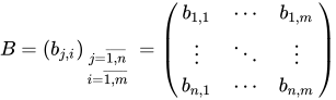of size ,

in which for all and .

Such a matrix is called the transposed matrix for and is denoted ,

sometimes (when there is no risk of confusion with differentiation) denoted ,

sometimes (when there is no risk of confusion with Hermitian conjugation) denoted .

Under transposition, the rows (columns) of the matrix become the columns (respectively, rows) of the matrix .

Obviously, .

For matrices over a ring , transposition is an isomorphism of - modules of matrices, since

,

, for any .

Diagonal Matrix[ | ]

A diagonal matrix is a square matrix all of whose elements, except those on the diagonal, are zero , sometimes written as:

Identity Matrix[ | ]

An identity matrix is a matrix that leaves any matrix (or vector) unchanged when multiplied by it, and it is a diagonal matrix with all diagonal elements equal to one:

It is most often denoted by I or E, or simply by 1 (or 1 in a special typeface).

The Kronecker symbol is also used to denote its elements, defined as:

when

Zero Matrix[ | ]

To denote the zero matrix — a matrix all of whose elements are zero (adding it to any matrix leaves that matrix unchanged, while multiplying it by any matrix gives the zero matrix) — one usually uses simply 0, or 0 in a special typeface, or a letter shaped like zero, for example .

Operations on Matrices

Operations on matrices

Addition of Matrices[ | ]

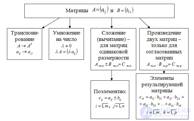
Only matrices of the same size can be added.

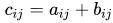
Addition of matrices is the operation of finding the matrix , all of whose elements are equal to the pairwise sum of the corresponding elements of the matrices and , that is, each element of the matrix is equal to

Properties of matrix addition:

• commutativity: A+B = B+A;
• associativity: (A+B)+C =A+(B+C);
• addition with the zero matrix: A + Θ = A;
• existence of the opposite matrix: A + (-A) = Θ;

All properties of linear operations replicate the axioms of a linear space, and therefore the following theorem holds:

The set of all matrices of the same size mxn with elements from a field P (the field of all real or complex numbers) forms a linear space over the field P (each such matrix is a vector of this space). However, mainly to avoid terminological confusion, in ordinary contexts matrices are, without real necessity for it (there being none in the most common standard applications) and without a precise clarification of the term's usage, generally avoided being called vectors.

Multiplication of a Matrix by a Number[ | ]

Multiplying a matrix by a number consists in constructing the matrix .

Properties of multiplying matrices by a number:

• multiplication by one: 1A = A;
• associativity: (λβ)A = λ(βA);
• distributivity: (λ+β)A = λA + βA;
• distributivity: λ(A+B) = λA + λB;

Multiplication of Matrices[ | ]

Multiplication of matrices (notation: , less often with the multiplication sign ) is the operation of computing the matrix , each element of which is equal to the sum of the products of the elements in the corresponding row of the first factor and the column of the second.

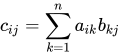
The number of columns in the matrix must match the number of rows in the matrix ; in other words, the matrix must be conformable with the matrix . If the matrix has dimensions , and has dimensions , then the dimensions of their product are .

Properties of matrix multiplication:

• associativity: (AB)C = A(BC);
• non-commutativity (in the general case): AB BA;
• the product is commutative when multiplying by the identity matrix: AI = IA;
• distributivity: (A+B)C = AC + BC, A(B+C) = AB + AC;
• associativity and commutativity with respect to multiplication by a number: (λA)B = λ(AB) = A(λB);

Multiplication of a Vector by a Matrix[ | ]

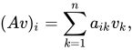
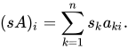
According to the usual rules of matrix multiplication, a column vector is multiplied by a matrix written to its left, while a row vector is multiplied by a matrix written to its right. Since the elements of a column vector or row vector can be written (as is usually done) using one index rather than two, this multiplication can be written as follows:

for a column vector v (yielding a new column vector Av):

for a row vector s (yielding a new row vector sA):

A row vector, a matrix, and a column vector can be multiplied together, giving a number (a scalar):

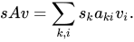
(Order matters: the row vector on the left, the column vector on the right of the matrix).

These operations form the basis of the matrix representation of linear operators and linear coordinate transformations (changes of basis), such as rotations, scalings, and mirror reflections, as well as (the last of these) the matrix representation of bilinear (quadratic) forms.

• When a vector of a real vector space is represented in an orthonormal basis (which is equivalent to using rectangular Cartesian coordinates), the corresponding column vector and row vector, which represent the set of components of the vector, will coincide (element-wise), differing only formally in their representation for the sake of correctness of matrix operations (that is, one is obtained from the other simply by the operation of transposition). When non-orthonormal bases are used, however (for example, oblique coordinates, or even just different scales along the axes), the column vector corresponds to the components of the vector in the primary basis, while the row vector — to components in the basis dual to the primary one (sometimes the space of row vectors is also referred to as a special space dual to the space of column vectors, the space of covectors).

Note that the usual motivation for introducing matrices and defining the operation of matrix multiplication (see also the article on matrix multiplication) is precisely to introduce them starting with the multiplication of a vector by a matrix (which is introduced based on basis transformations or, more generally, linear operations on vectors), and only afterward is the product of matrices associated with the composition of transformations. Indeed, if the new vector Av, obtained from the original vector v by a transformation representable as multiplication by the matrix A, is now transformed once more by a transformation representable as multiplication by the matrix B, giving B(Av), then, starting from the rule for multiplying a vector by a matrix given at the beginning of this section (using the associativity of multiplication of numbers and changing the order of summation), it is easy to see, as a result, the formula giving the elements of the matrix (BA), which represents the composition of the first and second transformations and coincides with the usual definition of matrix multiplication.

Complex Conjugation[ | ]

If the elements of the matrix are complex numbers, then the complex conjugate (not to be confused with the Hermitian conjugate! see below) matrix is equal to . Here is the number complex-conjugate to .

Transposition and Hermitian Conjugation[ | ]

Transposition has already been discussed above: if , then . For complex matrices, the Hermitian conjugate is more commonly used: . From the operator point of view on matrices, the transposed and Hermitian conjugate matrices are the matrices of the operator that is adjoint with respect to the scalar or Hermitian product, respectively.

Minors[ | ]

Trace: Trace of a Matrix

For a square matrix , the sum of the diagonal elements (i.e., the principal minors of the first order) is called the trace:

(other notations , , ).

Properties:

1. If and are defined, then .
2. The trace is an invariant of similarity transformations of a matrix, i.e., if is non-singular, then .
3. The trace equals the sum (of all, counted with multiplicity) of the eigenvalues of the matrix: . Moreover, for any (positive) integer , holds.

Determinant[ | ]

Determinant

Let the matrix be square, then the notation for the determinant is: . If the matrix , then

Permanent[ | ]

Permanent

Related Concepts[ | ]

Linear Combinations[ | ]

In a vector space, a linear combination of the vectors is called the vector

where are the expansion coefficients:

• if all the coefficients are equal to zero, the combination is called trivial,
• if at least one coefficient is nonzero, the combination is called nontrivial.

This makes it possible to describe the product of the matrices and in terms of linear combinations:

• the columns of the matrix are linear combinations of the columns of the matrix with coefficients taken from the matrix ;
• the rows of the matrix are linear combinations of the rows of the matrix with coefficients taken from the matrix .

Linear Dependence[ | ]

If some vector can be represented as a linear combination, one speaks of the linear dependence of that vector on the elements of the combination.

More precisely: a certain set of elements of a vector space is called linearly dependent if there exists a linear combination of the elements of this set that equals zero, or

where not all the numbers are zero; if no such nontrivial combination exists, then the given set of vectors is called linearly independent.

Linear dependence of vectors means that some vector of a given set is linearly expressed through the remaining vectors.

Each matrix represents a set of vectors (of the same space). Two such matrices are two sets. If every vector of one set is linearly expressed through the vectors of another set, then in the language of matrix theory this fact is described using the product of matrices:

• if the rows of the matrix linearly depend on the rows of the matrix , then for some matrix ;
• if the columns of the matrix linearly depend on the columns of another matrix , then for some matrix .

Properties[ | ]

Matrix Operations[ | ]

Addition and subtraction are allowed only for matrices of the same size.

There exists a zero matrix such that adding it to another matrix A does not change A, that is

All elements of the zero matrix are equal to zero.

Only square matrices can be raised to a power.

• Associativity of addition:
• Commutativity of addition:
• Associativity of multiplication:
• In general, matrix multiplication is non-commutative: . This property gives rise to the commutator of matrices.
• Distributivity of multiplication over addition:

  

  

• Given the properties listed above, matrices form a ring with respect to the operations of addition and multiplication.
• Properties of the matrix transpose operation:

  

  

  , if the inverse matrix exists.

  

  

Examples List of Matrices

This section collects the most important classes of matrices used in mathematics, science in general, and applied science in particular.

A matrix is understood to be a rectangular array of numbers called elements. Matrices have a long history of study and application, which has led to various ways of classifying them. The first group of matrices satisfies specific conditions and restrictions on their elements, including constant matrices. An important example of this kind of matrix is the identity matrix:

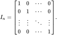
It is also denoted by the letter E. Other ways of classifying matrices are related either to their eigenvalues or to conditions expressed as matrix equations (relations). Finally, in many fields (in physics and in chemistry) matrices of a special form are encountered that are used exclusively in those fields.

Matrices Defined by Conditions on Their Elements[ | ]

The list of matrices given below is defined by conditions imposed on the elements of the matrices. Many of these properties turn out to apply only to square matrices. A square matrix has two diagonals: the main diagonal (running from the upper-left corner to the lower-right corner) and the anti-diagonal (running from the lower-left corner to the upper-right corner).

Matrices of General Form[ | ]

The matrices presented below are characterized by the fact that the conditions on their elements are described in terms of the matrix's structure. This includes the relative arrangement of nonzero elements, as well as invariance properties with respect to matrix transformations.

Name	Description	Remarks, explanations
Binary matrix	A matrix consisting of zeros and ones.	Synonyms: Boolean matrix, logical matrix.
Alternant matrix	A matrix whose elements are the values of functions at specified points.
Zero matrix	A matrix consisting entirely of zeros.
Anti-diagonal matrix	A square matrix all of whose elements outside the anti-diagonal are equal to zero.
Anti-Hermitian matrix	A square matrix with complex elements that maps to itself with a sign change under the Hermitian conjugation operation (that is, under complex conjugation of every element followed by transposition of the matrix),	Synonym of a skew-Hermitian matrix.
Antisymmetric matrix		Synonym of a skew-symmetric matrix.
Arrowhead matrix (English)	A square matrix all of whose nonzero elements belong to the first column, the first row, or the main diagonal.
Band matrix (English)	A square matrix all of whose nonzero elements are adjacent to the main diagonal.
Bidiagonal matrix (English)	A matrix all of whose nonzero elements lie on the main diagonal and on one of the sub- or superdiagonals.
Bisymmetric matrix	A square matrix that is symmetric both with respect to the main diagonal and with respect to the anti-diagonal.
Block diagonal matrix	A block matrix that has matrices only on the main diagonal.
Block matrix	A matrix partitioned into submatrices called blocks.
Block tridiagonal matrix (English)	A block matrix whose blocks are organized in the same way as those of a tridiagonal matrix.
Boolean matrix		synonym for a (0,1)-matrix, a binary matrix, and a logical matrix.
Cauchy matrix	A matrix each of whose elements has the form where and — are two injective sequences
Centrosymmetric matrix	A matrix that is symmetric with respect to its center, that is:
Conference matrix	A square matrix with zero elements on the diagonal and elements of the form +1 and −1 off the diagonal, such that — is the identity matrix.
Complex Hadamard matrix (English)	A matrix all of whose rows and columns are pairwise orthogonal to each other, and whose elements themselves are unimodular.
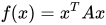
Positive semi-definite matrix	A square matrix with real elements such that the quadratic form is nonnegative for every nonnegative
Diagonally dominant matrix	A matrix whose elements satisfy the condition given here: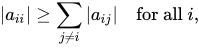
Diagonal matrix	A matrix all of whose elements outside the main diagonal are equal to zero.
Elementary matrix (English)	A matrix obtained from the identity matrix by means of elementary transformations.
Equivalent matrix (English)	A matrix obtained from another matrix by means of elementary row or column transformations.
Frobenius matrix	A matrix obtained from the identity matrix by shifting it and adding a new column.
Hermitian matrix, Hermitian self-adjoint matrix	A square matrix with complex elements that maps to itself under the Hermitian conjugation operation (that is, under complex conjugation of every element followed by transposition of the matrix),
Nonnegative matrix	A matrix all of whose elements are nonnegative.
Permutation matrix	A square matrix in which each column and each row contains exactly one 1, and all other entries are 0. It is the matrix representation of a permutation.
Generalized permutation matrix (English)	A square matrix with exactly one nonzero element in each row and each column.
Persymmetric matrix	A matrix that is symmetric with respect to the anti-diagonal:
Polynomial matrix	A matrix all of whose elements are polynomials.
Positive matrix	A matrix all of whose elements are positive.
Quaternion matrix	A matrix all of whose elements are quaternions.
Sign matrix (English)	A matrix all of whose elements equal 1, 0, or −1.
Signature matrix (English)	A matrix all of whose elements equal either 1 or −1.
Skew-Hermitian matrix	A square complex matrix that changes sign under Hermitian conjugation.	Same as an anti-Hermitian matrix.
Skew-symmetric matrix	A square matrix that changes sign under transposition,	Same as an antisymmetric matrix.
Skyline matrix (English)	A band matrix reorganized so as to reduce the storage space it occupies.
Sparse matrix	A matrix consisting almost entirely of zeros.	Algorithms for sparse matrices make it possible to process larger matrices than for dense ones
Sylvester matrix	A square matrix whose elements — are the coefficients of two polynomials.	A Sylvester matrix is nonsingular if and only if the two polynomials are coprime.
Symmetric matrix	A square matrix that coincides with its transpose: ().
Toeplitz matrix	A matrix in which the same elements appear along each diagonal.
Triangular matrix	A matrix all of whose elements above the main diagonal are zero (lower triangular matrix), or a matrix all of whose elements below the main diagonal are zero (upper triangular matrix).
Tridiagonal matrix	A matrix all of whose nonzero elements lie on three diagonals: the main diagonal, the first one above it, and the first one below it.
Unitary matrix	A square complex matrix whose inverse equals its Hermitian conjugate,
Special unitary matrix	A unitary matrix whose determinant equals one
Vandermonde matrix	A matrix whose rows (or columns) consist of successive powers: 1, a, a2, a3, …, an
Walsh matrix (English)	A square matrix whose size is a power of two, consisting of elements +1 or −1.
Z-matrix	A matrix all of whose off-diagonal elements are less than zero.
Hankel matrix	A square matrix in which the elements on each anti-diagonal are equal.

Constant Matrices[ | ]

The matrices presented below are characterized by the fact that their elements are the same for all possible matrix sizes.

Name	Description	Conditions on elements	Remarks
Exchange matrix	A binary matrix with ones on the anti-diagonal and all other elements zero.		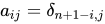See Permutation matrix.
Hilbert matrix			See Hankel matrix.
Identity matrix	A square matrix with ones on the main diagonal and all other elements equal to zero.
Lehmer matrix		aij = min(i, j) ÷ max(i, j)	See positive symmetric matrix.
Matrix of ones	A matrix all of whose elements are one.
Pascal matrix	A matrix consisting of the elements of Pascal's triangle.
Pauli matrix	A block matrix consisting of 2 × 2 blocks, each of which is a complex Hermitian and unitary matrix.
Redheffer matrix		aij = 1, if i is divisible by j or if j = 1; otherwise, aij = 0.	See (0, 1)-matrix.
Shift matrix	A matrix with ones on one of the off-diagonals, and all other elements zero.	or	Multiplying by this matrix shifts the elements by one position.
Zero matrix	A matrix all of whose elements are zero.

Transformed Matrices[ | ]

• Inverse matrix
• Transpose matrix
• Hermitian conjugate (adjoint) matrix
• Adjugate matrix

Matrices Satisfying Conditions on Products or Inverses[ | ]

Matrices Used in Graph Theory

• Adjacency matrix
• Biadjacency matrix
• Degree matrix
• Edmonds matrix
• Incidence matrix
• Kirchhoff matrix (Laplacian matrix)
• Seidel adjacency matrix
• Tutte matrix

Matrices Used in Physics[ | ]

• Cabibbo-Kobayashi-Maskawa matrices
• Dirac gamma matrices
• Pauli matrices
• Gell-Mann matrices
• S-matrix
• Density matrix

Square Matrix and Related Definitions[ | ]

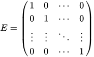
If the number of rows of a matrix equals the number of columns, such a matrix is called square.

For square matrices there exists an identity matrix (an analog of the number one for multiplication) such that multiplying any matrix by it does not affect the result, namely

In the identity matrix, ones appear only on the main diagonal, while all other elements are equal to zero

For some square matrices one can find a so-called inverse matrix. The inverse matrix is such that if a matrix is multiplied by its inverse, the result is the identity matrix:

The inverse matrix does not always exist. Matrices for which an inverse matrix exists are called non-singular (or regular), and those for which it does not are called singular (or degenerate). A matrix is non-singular if all of its rows (columns) are linearly independent as vectors. The maximum number of linearly independent rows (columns) is called the rank of the matrix. The determinant of a matrix is the value of the normalized skew-symmetric (antisymmetric) multilinear form of valence on the columns of the matrix. A square matrix over a number field is singular if and only if its determinant equals zero.

The Ring of Matrices[ | ]

From the above properties of matrix addition and multiplication (associativity and commutativity of addition, distributivity of multiplication, existence of a zero matrix and of an additive inverse matrix) it follows that square n by n matrices with elements from any ring R form a ring isomorphic to the ring of endomorphisms of the free module Rn. This ring is denoted by or . If R is a commutative ring, is also an associative algebra over R. The determinant of a matrix with elements from a commutative ring can be computed by the usual formula, and the matrix is invertible if and only if its determinant is invertible in R. This generalizes the situation for matrices with elements from a field, since in a field every element except zero is invertible.

Matrices in Group Theory[ | ]

Matrices play an important role in group theory. They are used in constructing general linear groups, special linear groups, diagonal groups, triangular groups, and unitriangular groups.

A finite group (in particular, a symmetric group) can be (isomorphically) modeled by permutation matrices (containing only «0» and «1»),

for example, for : , , , , , .

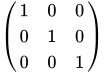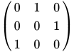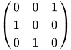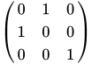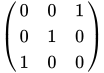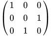The field of complex numbers can be (isomorphically) modeled over the field of real numbers:

for the matrix analogs 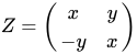, , 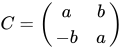where ;

corresponds to ;

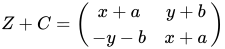corresponds to ;

corresponds to ;

;

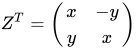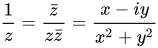for corresponds to 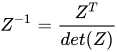for ;

corresponds to .

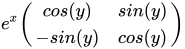In particular, for ,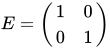

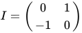
corresponds to ,

where .

Remark. The model has an automorphism , that is

The division ring of quaternions can be (isomorphically) modeled over the field of real numbers:

for the matrix analog 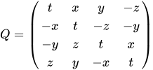, where .

In order for the quaternion to correspond to the matrix ,

where , , , ,

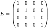
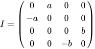
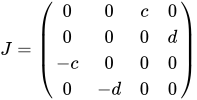
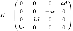
one can introduce basis elements

, , , .

The parameters must satisfy the conditions: and .

There exist 8 solutions (8 representations).

See Also

• Matrix norm
• Determinant of a matrix
• Eigenvectors, eigenvalues, and eigenspaces
• Array — a data type in programming that corresponds to a matrix (multidimensionality is achieved through nested arrays).
• Sparse array — one of the computer representations of sparse matrices.
• Linear matrix inequalities — a tool for solving control law synthesis problems.
• Lambda matrix
• Jordan normal form
• List of matrices