Lecture
Speaking of statistical methods of recognition, we assume the establishment of a relationship between the assignment of an object to a particular class (image) and the probability of error when solving this problem. In some cases, this comes down to determining the posterior probability of the object being in the image  provided that the attributes of this object took on the values
  . Let's start with the Bayes decision rule. By Bayes formula

Here  - a priori probability of presentation to object recognition
  th image:

 .
.
For each 
 ,
,
with signs of continuous measurement scale
 ,
,
with signs with a discrete measurement scale
 .
.
At continuous values of signs  is a probability density function, with discrete - probability distribution.
Distributions describing different classes, as a rule, "intersect", that is, there are such characteristic values  at which
 .
.
In such cases, recognition errors are inevitable. Naturally, there are no interesting cases when these classes (images) in the chosen feature system  indistinguishable (with equal a priori probabilities, solutions can be chosen by randomly assigning an object to one of the classes in an equiprobable manner).
In general, one should strive to choose the decision rules in such a way as to minimize the risk of loss in recognition.
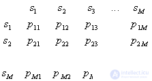
The risk of loss is determined by two components: the probability of recognition errors and the magnitude of the "penalty" for these errors (losses). Matrix of recognition errors:
 ,
,
Where  - the probability of correct recognition;
 - the probability of erroneous assignment of the object
  th image to
  -mu (
-mu (  ).
).
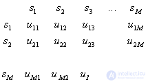
Loss matrix

 ,
,
Where  - "award" for the correct recognition;
 - "penalty" for the erroneous assignment of an object
  th image to
  -mu (
-mu (  ).
).
It is necessary to construct a decision rule in such a way as to ensure a minimum of expected losses (minimum of average risk). This rule is called Bayesian.
We divide the sign space  on
on  disjoint areas
  each of which corresponds to a particular image.
The average risk with hit implementations  th image in the area of other images is equal
 ,
,  .
.
Here it is assumed that all components  have a continuous scale of measurements (in this case it is not fundamental).
Magnitude  can be called a conditional average risk (provided that an error is made in recognizing an object
  th image). The total (unconditional) average risk is determined by
Decision rules (partitioning methods  on
on 
 ) form a multitude
  . The best (Bayesian) decisive rule is that which provides minimal average risk.
  where
where  - the average risk in applying one of the decisive rules included in
  .
.
Consider the simplified case. Let be  , but
, but  (
(  ). In this case, the Bayes decision rule ensures a minimum of the probability (average number) of recognition errors. Let be
  . The probability of an error of the first kind (the object of the 1st image is assigned to the second image)
 ,
,
Where  - probability of error of the second kind
 .
.
Average errors
 .
.
Because  then
then  and
and  . Clearly at least
  will have a minimum if the integrand in the region
  will be strictly negative that is in
 . In the area of
  the opposite inequality must be satisfied. This is the Bayes decision rule for the case under consideration. It can be written differently:
  ; magnitude
  considered as a function of
  called likelihood
  at this
  , but
, but  - likelihood ratio. Thus, the Bayes decision rule can be formulated as a recommendation to choose a solution.
  if the likelihood ratio exceeds a certain threshold value that does not depend on the observed
  .
.
Without special consideration, we note that if the number of recognized classes is more than two (  ), the decision in favor of the class (image)
  is accepted in the field
  in which for all
 .
.
Sometimes with a low accuracy of a posteriori probability estimation (small volumes of a training sample), so-called randomized decision rules are used. They consist in the fact that an unknown object is attributed to a particular image not according to the maximum a posteriori probability, but in a random way, in accordance with the a posteriori probabilities of these images  . This can be implemented, for example, in the manner shown in Fig. 18.


Fig. 18. Illustration of randomized decision rule
After calculating the posterior probabilities of belonging of an unknown object with parameters  each of the images
  ,
,  , a straight line length of the unit is divided into
  intervals with numerically equal lengths
  , and each interval is associated with this image. Then, using a random (pseudo-random) number sensor, uniformly distributed on
  , generate a number, determine the interval in which it fell, and assign the recognizable object to the image to which the given interval corresponds.
It is clear that such a decision rule cannot be better than Bayesian, but for large values of the likelihood ratio is not much inferior to it, and in implementation it can be quite simple (for example, the nearest neighbor method, which will be discussed later).
Bayesian decision rule is implemented in computers mainly in two ways.
1. Direct calculation of a posteriori probabilities
 ,
,
Where  - vector of values of parameters of a recognizable object and selection of a maximum The decision is made in favor of the image for which
  as much as possible. In other words, the Bayes decision rule is implemented by solving the problem
  .
.
If we go to further generalization and assume the existence of a loss matrix of a general form, then the conditional risk can be determined by the formula  ,
,  . Here the first member defines the "encouragement" for correct recognition, and the second - the "punishment" for the mistake. The Bayesian decision rule in this case is to solve the problem.

2. "Topographic" area definition  which hit vector
  feature values describing a recognizable object.
This approach is used in cases where the description of areas  quite compact, and the procedure for determining the area in which it fell
  is simple. In other words, it is natural to use this approach when computationally it is more efficient (simpler) than direct calculation of a posteriori probabilities.

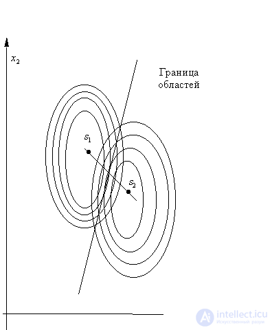
Fig. 19. Bayesian decision rule
for normally distributed attributes
with equal covariance matrices
So, for example (we will not give the proof), if there are two classes, their prior probabilities are the same,  and
and  - normal distributions with the same covariance matrices (differ only in the vectors of the means), then the Bayesian dividing boundary is the hyperplane. It is remembered by the values of the coefficients of the linear equation. When recognizing an object, the values of attributes are substituted into the equation
  of this object and by the sign (plus or minus) of the obtained solution the object is referred to
  or
or  (Fig. 19).
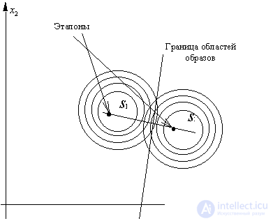
If y classes  and
and  covariance matrices
  and
and  not only the same, but also diagonal, the Bayesian solution is to assign an object to that class, the Euclidean distance to the standard of which is minimal (Fig. 20).

Fig. 20. Bayesian decision rule
for normally distributed attributes
with equal diagonal covariance matrices
(elements of the diagonals are the same)
Thus, we are convinced that some decision rules, previously considered by us as empirical (deterministic, heuristic), have a very clear statistical interpretation. Moreover, in some specific cases, they are statistically optimal. We will continue the list of similar examples by further consideration of statistical recognition methods.
We now turn to methods for estimating the distribution of values of features of classes. Knowledge  is the most universal information for solving problems of recognition by statistical methods. This information can be obtained in two ways:
define in advance  for all
  and
and  ;
;
define  at each act of recognition of a particular object, the attributes of which have values
  .
.
Each of these approaches has its advantages and disadvantages, depending on the number of features, the size of the training sample, the availability of a priori information, etc.
Let's start with the local version (definitions  in the vicinity of a recognizable object).
Comments
To leave a comment
Pattern recognition
Terms: Pattern recognition