Nearest Neighbor Method for Static Pattern Recognition

Here the idea is that around a recognizable object volume cell is built . At the same time, an unknown object belongs to that image, the number of training representatives of which in the constructed cell turned out to be the majority. If we use statistical terminology, then the number of image objects trapped in this cell characterizes the estimate of the volume averaged probability density .

To assess the averaged need to solve the question of the relationship between volume cells and the number of objects of one or another class (image) that fell into this cell. It is reasonable to assume that the smaller the more subtly be characterized . But at the same time, the fewer objects will fall into the cell of interest, and therefore, the less reliable the estimate . With an excessive increase reliability of an assessment increases , but the subtleties of its description are lost due to averaging over too large a volume, which can lead to negative consequences (an increase in the probability of recognition errors). With a small amount of training sample It is advisable to take extremely large, but to ensure that within the cell density little changed. Then their averaging over a large volume is not very dangerous. Thus, it may well happen that the cell volume relevant for one value may not be suitable for other cases.

The following procedure is proposed (for now, we will not take into account the belonging of an object to a particular image).

In order to evaluate based on a training set containing objects, center the cell around and increase its volume as long as it does not contain objects where there is some function from . These objects will be closest neighbors . Probability vector hits to the area determined by the expression .

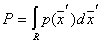This is a smoothed (averaged) density distribution. . If you take a sample of objects (by a simple random selection from the general population), of them will be inside the area . Probability of hitting of objects in described by a binomial law having a pronounced maximum around the mean . Wherein is a good estimate for .

If we now assume that so small that inside it changes slightly, then

,

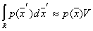Where - area volume , - point inside .

Then . But , Consequently, .

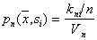
So, the assessment density is the value

. (*)

Without proof we give the statement that the conditions

and (**)

are necessary and sufficient for convergence to in probability at all points where the density continuous.

This condition is satisfied, for example, .

Now we will take into account the belonging of objects to one or another image and try to estimate the posterior probabilities of the images.

Suppose we place a volume cell around and grab the sample with the number of objects , of which belong to the image . Then according to the formula estimation of joint probability there will be a magnitude

,

but

.

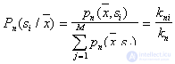Thus, the posterior probability estimated as the fraction of the sample in the cell related to . To minimize the error level, you need an object with coordinates attributed to the class (image), the number of objects of the training sample of which is maximum in the cell. With such a rule is Bayesian, that is, it provides a theoretical minimum of the probability of recognition errors (of course, the conditions ).