
Lecture
Classification of software quality models and metrics. The software of an information system consists of a set of various software products, tied together by the IS designer (developer) into a single system of software tools (environment), whose interaction is ensured by the necessary program interface. Thus, the quality of the whole software depends on the reliability of the software products included in it [21, 22, 23, 25, 30, 33, 47].
Models and metrics for evaluating software product quality are a system of measurements of program quality. These measurements can be carried out at the level of software product quality criteria or at the level of individual quality characteristics. In the first case, the measurement system allows programs to be compared directly by quality; however, the measurements themselves cannot be carried out without subjective assessments of the software product's properties. In the second case, the characteristics can be measured objectively and reliably, but the overall quality assessment of the software product will be tied to a subjective interpretation of the resulting estimates.
In the study of software product quality assessment models and metrics, two main directions are distinguished:
the search for models and metrics characterizing the most specific properties of programs, i.e., metrics for evaluating the software product itself;
the use of models and metrics to evaluate the technical characteristics and factors of software product development, i.e., models and metrics for evaluating the conditions of software product development.
By the type of information obtained when evaluating software product quality, all the main models and metrics can be divided into three groups:
1) models and metrics that evaluate the deviation from the norm of the characteristics of the source design materials. They establish the completeness of the specified technical characteristics of the source code;
2) models and metrics that make it possible to predict the quality of software products under development. They are defined over the set of possible solution variants for the task at hand and their implementations, and determine the quality of the software product that will be achieved;
3) models and metrics by which a decision is made on the compliance of the final software with the specified requirements. They make it possible to assess the compliance of the development with the specified requirements:
At present, several hundred program metrics are used in world practice. Existing quality assessments of software products can be grouped into six directions:
1) assessments of the topological reliability of the software, allowing failure situations to be predicted;
2) assessments of software reliability, allowing failure situations to be predicted;
3) assessments of software product performance and the improvement of its efficiency by identifying design errors;
4) assessments of the level of language tools and their application;
5) assessments of the difficulty of perceiving and understanding program texts, oriented toward psychological factors significant for the maintenance and modification of programs;
6) assessments of programmer productivity for predicting software product development timelines and planning work on software creation.
Analysis of the technological experience of leaders in software product production shows how costly the imperfection of an unscientific forecast of feasibility, labor costs, complexity, inflexible control, and management of development, among other things, can be — indicating the absence of end-to-end methodological support and ultimately leading to the software product's non-compliance with user and/or standard requirements, and to a subsequent painful and labor-intensive rework. These circumstances require careful selection of methods, models, and techniques for assessing software product quality, taking into account the limits of their applicability for various life cycles and within a single life cycle, establishing the order of their joint use, applying redundant multi-model study of the same indicators to increase the reliability of current assessments, and accumulating and integrating heterogeneous metric information for making timely production decisions and the final certification of the software product.
Analysis of models. Let us give a brief analysis of the models and metrics that have proven themselves well in evaluating software product quality and are suitable for predicting and stating various indicators of software product complexity and reliability.
Mills model. This model belongs to the class of static models used by programmers or testers in the process of developing, testing, and certifying a software product. Static models differ from dynamic models primarily in that they do not take into account the time of occurrence of errors during testing and do not use any assumptions about the behavior of the risk function. These models are built on a solid statistical foundation.
Using the Mills model requires that, before testing begins, a certain known number L of specific errors be artificially introduced into the program. Errors are introduced randomly and recorded in the artificial error log. The specialist conducting the testing knows neither the number nor the nature of the artificially introduced errors until the moment the reliability indicators are evaluated using the Mills model.
The basic assumption underlying the model is that the distribution of artificially introduced errors is considered to be the same as the distribution of the program's own errors, and, consequently, the probability of detecting both the program's own errors and the seeded ones is the same. Testing of the program is then begun. During testing of the program, statistics on errors are collected over a period of time. Suppose S errors are detected. At the moment reliability is evaluated using the artificial error log, all detected errors are divided into the program's own and artificial ones:

Where l is the number of artificially introduced errors among those detected; V is the number of the program's own errors among those detected.
Then, in accordance with the maximum likelihood method, the estimate of the number of errors remaining in the software (the initial number of errors) will be the following value:

The second part of the Mills model is concerned with testing the hypothesis regarding the value of N. Suppose the program has R own errors; let us additionally introduce L errors into it. During testing, all L introduced errors and r own errors were detected. Then, according to formula (3.6), we assume that the program initially had N = r errors. The probability with which this assumption can be made can be estimated using the following relations:

Thus, the value of P is a measure of confidence in the model and shows the probability of how correctly the value of N has been found. These two related relations form a useful error model: relation (3.6) predicts the possible number of errors originally present in the program, while relation (3.7) is used to establish the confidence level of the prediction.
However, formula (3.7) for calculating P cannot be used in the case when not all of the artificially introduced errors have been detected. When evaluating reliability in the case where l artificially introduced errors are detected (l

For example, if it is asserted that there are no errors in the program, and by the time reliability is evaluated five out of 10 artificially introduced errors have been detected and not a single own error has been detected, then the probability that the program indeed has no errors is:
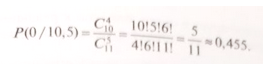
However, if, given the same results, it is asserted that the program has one own error, then the probability of this event is:

If, under the same initial conditions, the reliability estimate is made at the moment when eight of 10 artificial errors have been detected and no other errors have been detected, then the probability that the program had no errors increases to 0.73. The Mills model can be used to estimate the number of initial errors N after each error found. It is proposed that throughout the entire testing period the number of errors found and the current value of N be marked on a graph.
The advantages of the model are the simplicity of applying the mathematical apparatus, clarity, and the possibility of using it directly during testing; the disadvantages are the need to introduce artificial errors (this process is poorly formalized) and the rather loose assumption about the value of R, which is based only on the intuition and experience of the person conducting the assessment, i.e., a strong influence of the subjective factor is allowed. A significant drawback of this model is also the assumption that the distribution of the program's own errors and the artificially introduced errors is the same, which cannot be verified, especially at later stages of program development, when many simple errors (for example, various omissions) have already been eliminated and the most difficult to detect errors remain.
Jelinski-Moranda model. This is one of the first and simplest models of the classical type, which served as an impetus for further developments in this area. The model was used in the development of software products for critical projects. The Jelinski-Moranda model is intended for use during the testing of a software product.
This model is built on the basis of a number of assumptions:
the detection rate λ(t) is proportional to the current number of errors in the program, i.e., to the number of remaining errors;
all errors are equally likely and their occurrence is independent;
each error has the same order of severity;
the time to the next failure (error) is exponentially distributed;
the software operates in an environment close to the real one;
errors are continuously corrected without introducing new ones into the software;
λ(t) = const in the interval between two neighboring errors. In accordance with these assumptions, the error detection rate in the software can be represented as

where 7 is the arbitrary time between the detection of the (i - 1)-th and i-th errors; K is an unknown coefficient; B is the unknown total number of errors in the software product.
Consequently, if (i - 1) errors have been detected during time t, then [B - (i - 1)] errors still remain in the software product. Setting Xi = ti- ti-1 (i = 1,2,..., n) and taking into account the assumption that λ(t)= const in the interval between the detection of the (i - 1)-th and i-th errors, the values of Xi can be considered to have an exponential distribution. To obtain estimates of the number of errors in the program  (including the remaining errors) and of the unknown coefficient K, the following relations are used:
To obtain an estimate after detecting n errors. Let us set =m-1, where m ≥n + 1 is the number of predicted (including as yet undetected) errors. We calculate the value 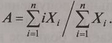 We check the condition
  Then, successively varying m, we find the values of two functions: the function
  and the function
  Next we calculate the values of the absolute differences
  . Finding the first minimum of the absolute difference with respect to m, we determine the value of m as the best integer solution of the equation
To obtain the value  after detecting n errors. We calculate the unknown parameter using the formula
From the values found and , estimates of the following unknown parameters can be determined:
the rate of error occurrence in the software product after the i-th error has already been detected in it - 
the mean time to the occurrence of the (i + 1)-th error in the software product - 
the time until the completion of software product testing - 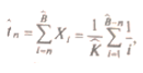 , where n is the number of errors identified as of the current day of software product testing
Schick-Wolverton model. This model is built for developers and testers to evaluate the dependence of software product reliability on certain specific parameters. It is a modification of the Jelinski-Moranda model for the case where more than one error can occur in the interval under consideration. The Schick-Wolverton model is based on the assumption that the error detection rate is proportional not only to the number of errors in the program, but also to the testing time, i.e., the probability of detecting errors increases over time. In this model the observed event is the number of errors detected in a given time interval, rather than the waiting time for each error, as was the case for the Jelinski-Moranda model.
Simple exponential model. The main difference between this model and the Jelinski-Moranda model is that assumption 7 is removed, and thus the risk function ceases to be piecewise constant. Developers and testers assume that the risk function is proportional to the number of errors remaining in the software product, minus the errors already detected.
Lipow models. These models are a generalization of the Jelinski – Moranda and Schick – Wolverton models respectively and are used by developers or testers in the process of developing, testing, and certifying a software product. Unlike the previous ones, they allow more than one error to occur within a single program testing interval, and also permit correction of not all the errors detected in that interval. Lipow modified the Mills model by considering the probability of detecting an error when using different numbers of tests. The Lipow model supplements the Mills model, making it possible to estimate the probability of detecting a certain number of errors by the time of the assessment.
Basin model. This is a software product reliability model intended for developers and testers in the process of testing a software product and detecting errors. Testers use this model in the following way: suppose a software product contains Nk instructions. From this number, n instructions are randomly selected, into which errors are introduced. Then, for testing, r instructions are randomly selected. If during testing v own errors and m introduced errors are detected, then a maximum likelihood estimate is made of the number B6 of errors contained in the program before testing began. When using this procedure, the tagging level (the average number of tagged errors) should be greater than 20 in order to be confident of the objectivity of the estimates obtained. These procedures can be acceptable at any stage after the programmers' coding.
Bell-LaPadula security model. This is one of the first security models, which subsequently became the most frequently used. It was developed by David Bell and Leonard LaPadula for developers and designers and was used in the process of designing and modeling computer operation. All system components are divided into objects and subjects. The concept of a secure state is introduced, and it is proved that if every transition preserves the secure state, i.e., transfers the system from a secure state to a secure state, then, according to the principle of induction, the system is secure.
In the Bell-LaPadula model about 20 functions (operation rules) are defined, performed when modifying the components of the access matrix, when requesting and gaining access to an object (for example, when opening a file), and when creating and deleting objects; in doing so, for each function it is proved that it preserves (in accordance with the definition) the secure state. Only a few developments of secure systems used the functions proposed by Bell and LaPadula; more often, their own functions were used, developed on the basis of the functions of the Bell-LaPadula model. Therefore, nowadays, when the Bell-LaPadula model is mentioned, only the simple security condition and the property of restriction are meant, and not the functions that form the basis of the model and their proofs.
Geometric models. There are three main geometric models: the first and third were proposed by P. B. Moranda (the first is a modification of the Jelinski-Moranda model discussed earlier); the second, proposed by M. Lipow, extends the first.
In the first model it is assumed that the initial number of errors in the program B is a non-fixed (unbounded) quantity: moreover, not all errors are equally probable. It is also assumed that as debugging proceeds it becomes increasingly difficult to detect errors, and thus the software product is never freed of errors. The main initial premises are:
the total number of errors is unlimited;
the detection of errors is not equally probable;
error detection is a process independent of the errors themselves;
the software product operates under conditions close to real ones;
The rate of error detection forms a geometric progression, and the rate in the interval between the occurrences of errors is constant.
The third geometric model is proposed for the case when error reports arrive periodically. As in the previous model, only the total number of errors identified in each testing interval is required. However, unlike the previous geometric models, it is assumed that all testing intervals have the same length, measured in a day, a week, a month, etc. The model is applicable when the length of the interval is small compared to the testing time.
Schneidewind model. This model is built for developers and testers and includes the third geometric model as a special case. The main approach consists in the assumption of a stronger influence of the occurrence of later errors on the error prediction process. The main assumptions:
independence of the occurrence of errors in different intervals;
the number of errors detected decreases from interval to interval;
all intervals have the same length (day, week, month, etc.);
the error detection rate is proportional to the number of errors present at a given moment in time.
Musa model. The most developed to date are the continuous empirical reliability models (CERM) of a software product, intended for evaluating the reliability of a real-time software product. It is important to take into account the specific, particular properties and operating conditions of a software product of a given type, and even of individual developments of the software tool
The following definitions are used to build a CERM:
program reliability - the property of a program to operate failure-free under specified conditions for a specified period of time;
failure - an impermissible deviation of the characteristics of the program's operating process from those required;
error - a defect in the program that leads to a failure.
Musa's CERM is intended mainly for predicting the behavior of a program once it is put into operation. The Musa model takes into account two types of operating time:
total time t, which is counted during the development of the program up to the control point at which the reliability assessment is performed;
operational time t, representing the time of program use planned from the control point onward, on the assumption that no error correction will take place.
In the Musa model, for the operating time t it is assumed that:
1) the failure rate is proportional to the number of uncorrected errors;
2) the rate of change in the number of corrected errors, measured relative to operating time, is proportional to the failure rate.
The coefficient of proportionality in the Musa model is called the error reduction factor. It accounts for three types of defects, each proportional to the failure rate for the following reasons:
an increase in the number of defects due to the appearance of new errors in the process of correcting old errors;
the detection of an error that has not yet manifested itself, during program analysis carried out after a defect associated with it was found during testing;
the presence of failures whose cause cannot be found, and, consequently, the impossibility of correcting the errors that caused these failures.
The total number of errors detected and corrected is described by an exponential function of the total operating time t:

where No is the initial number of errors in the program (No can be estimated using another model that allows its value to be determined from data obtained during testing, for example the Shooman model); C is the test compression factor, which accounts for the deviation of the software product's test conditions from real ones; Mo is the total number of failures that may occur during the maintenance of the software; T0 is the mean time between failures at the start of testing.
During testing, the execution time of the program (the test run) up to the next failure is recorded. It is assumed that not every error in the software product can cause a failure, so more than one error may be detected during program execution before the next failure. It is assumed that over the entire life cycle of the software product Mo failures may occur, and in the process all No errors present in the software product before testing began will be detected.
The main parameters of the Musa model, Mo and To, are initially estimated from the characteristics of the software product itself, i.e., from a rough reliability prediction. Once information on the intervals between failures becomes available, the estimates of the parameters Mo and To are refined using the maximum likelihood method.
One of the advantages of the Musa model is the ability to use calendar time, which allows long-term planning during the development and operation of software tools; the drawback is the need for a large amount of a priori information.
Nelson model. This model was developed taking into account the basic properties of machine programs and uses probability theory methods only in cases where it is impossible to obtain complete information about a given factor (for example, when answering the question of which set of input data should be used for the next program run). All the approximations adopted in the model are clearly defined, and the limits of their applicability are known. Since the Nelson model is based on the properties of the software product, it allows further development through a more detailed description of other aspects of reliability. Some of the generalizations obtained from the model can be considered in the context of studying the software product's security problem. These features of the model allow it to be regarded as a direction within the mathematical theory of software product reliability, rather than as a simple reliability model.
The model gives the following mathematical definition of the reliability of a machine program: «The reliability of a program is the probability of failure-free execution of n program runs». Therefore, a run is a single trial of the software product.
Sequential analysis based on Wald's model. The assumption is introduced that if the probability of a successful run P lies in a sufficiently small neighborhood of the point Pa, then the risk of making an incorrect decision is acceptably small. Here, an incorrect decision is understood to mean the decision to reject a reliable software product or to accept an unreliable software product. Before testing begins, the programmer testing the software product must specify the following values:
the minimum acceptable probability of failure-free operation of the software product Pmin;
the probability Pmax, at which they are almost certain that the software product will pass the trials;
the probability of a type I error, i.e., the probability of rejecting a reliable software product;
the probability of a type II error, i.e., the probability of accepting an unreliable software product.
Halstead's model. This model is aimed at assessing complexity as a first step toward the purposeful reduction of the software product's complexity. Halstead's approach consists in determining the following indicators for any program:
the number of distinct operators n1;
the number of distinct operands n2;
the total number of all operators N1;
the total number of all operands N2;
the program vocabulary n;
the implementation length N.
From this data, the theoretical length of the program is determined, and accordingly the program volume, the potential volume of the program, and the potential volume of the program (in bits).
An important metric is the program level, defined as the ratio of the potential volume to the volume.
The language level metric makes it possible to quantitatively assess the advantages of a higher-level programming language compared with its predecessors. Another of the metrics proposed by Halstead makes it possible to estimate the time spent developing the software product. Halstead's complexity assessment of a program does not account for all the characteristics of program complexity. A program with a complex graph structure and a linear program that have the same volume are considered to have the same complexity, which is incorrect.
The complexity of the program itself depends on the data structures; the control structures determined by the program's logic; the correct partitioning into modules; the internal connections of each module; and the intermodule connections in the program, i.e., in the terminology of measurement theory, it is a latent, or hidden, variable, as opposed to indicator variables, which can be measured directly.
Duane model. This model was proposed to assess the growth of software product reliability. It considers the ratio of the error detection rate to the total testing time. The assumptions underlying the model are: the detection of all errors is equally probable and their severity is the same; the occurrence of errors is an independent process; the total number of errors detected by an arbitrary point in time is distributed according to the Poisson law. Implementing this model requires knowledge only of the times at which errors occur.
Model proposed by IBM specialists. While the consumer is using the current version of the software product, the developer, as a rule, carries out active maintenance of the version, i.e., continues to refine the version of the software product delivered to the consumer without waiting for complaints about it. Moreover, this refinement may also include creating additional functions for the given software product. From a certain point, when the developer considers its tasks finally completed, passive maintenance begins, i.e., at this stage refinement is carried out only at the user's request. Using the reliability models presented earlier, it is possible to estimate the number of errors remaining after testing in the first version of the software product delivered to the customer. It is notable that practically all models give a nonzero number of these errors.
During the maintenance of the software product, a significant number of new errors are introduced into its next version along with additions and changes, which leads to subsequent corrections in the next version. An attempt to predict such corrections from version to version was undertaken by developers at the American company IBM, based on a large volume of experimental data accumulated during the maintenance of the OS/360 operating system. The model they proposed is based on observing the history of the software product system's development and on the hypothesis of the statistical stability of the relationships between certain parameters characterizing different versions of the system. The main unit for measuring the complexity of the software product here is the program module. Rules for formatting modules were standardized.
Corcoran's model. Developers and testers applying this model should know the following:
the model accounts for different failure probabilities for different sources of errors and, accordingly, different probabilities of their correction;
the model uses parameters such as the result of only N trials, in which Ni errors of type i are observed;
the detection of an error of type i during N trials occurs with probability ai.
Shooman's model. It belongs to the dynamic discrete-time models, for which data are collected during testing of the software product over fixed or random time intervals. The model assumes that testing is carried out in several stages. Each stage consists of executing the program on the full set of test data developed. Detected errors are recorded but not corrected. At the end of the stage, quantitative reliability indicators are calculated, the errors found are corrected, the test suites are adjusted, and the next testing stage is carried out. Shooman's model assumes that the number of errors in the program is constant and that no new errors are introduced during correction. The rate of error detection is proportional to the number of remaining errors.
Metrics. McCabe's metric. The main complexity metric is proposed to be the cyclomatic complexity of the program graph, otherwise known as McCabe's cyclomatic number, which characterizes the effort required to test the program. To calculate the cyclomatic number λ (G) testers use the number of arcs of the directed graph G, the number of vertices, and the number of connected components of the graph. In essence λ (G) determines the number of linearly independent circuits in a strongly connected graph. In other words, McCabe's cyclomatic number shows the required number of passes to cover all the circuits of a strongly connected graph, or the number of test runs of the program needed for exhaustive testing according to the «every branch executes» criterion
Myers' metric. It is an extension of McCabe's metric. The essence of the approach lies in representing the program complexity metric as the interval  . For a simple predicate h = 0, and for n-ary predicates h = n - 1. This metric makes it possible to distinguish between programs represented by identical graphs. Unfortunately, information on the results of using this method is unavailable, so nothing can be said about its applicability.
Knot count metric. This program complexity metric (authors: M. Woodward, M. Hennell and D. Hedley) is aimed at analyzing programs whose creation used unstructured coding in languages such as assembly language and Fortran. In the program graph, where each statement corresponds to a vertex, a knot (crossing point of arcs) arises when control transfer goes outside the pair formed by the start and end vertices. The number of knots in the program graph provides a characteristic of the program's unstructuredness.
Gilb's metric. This is one of the simplest, yet fairly effective, estimates of software product complexity. The logical complexity of a program is defined as the program's saturation with IF-THEN-ELSE type expressions. Two characteristics are introduced here: CL — the absolute complexity of the program, characterized by the number of conditional statements; cl — the relative complexity of the program, characterized by the program's saturation with conditional statements, i.e., cl is defined as the ratio of CL to the total number of statements. By supplementing Gilb's metric with the characteristic of the maximum nesting level of a statement, CLI, it is possible not only to refine the analysis of IF-THEN-ELSE type statements, but also to successfully apply Gilb's metric to the analysis of loop constructs.
Boundary value metric. This is an estimate of program complexity using the boundary value method. To estimate program complexity, let us introduce several additional concepts related to the program graph. Let G = (V, E) be a directed program graph with a single start vertex and a single end vertex. In this graph, the number of arcs entering a vertex is called the negative degree of the vertex, and the number of arcs leaving a vertex is called the positive degree of the vertex. The set of graph vertices can then be divided into two groups:
1) vertices whose positive degree is not greater than 1;
2) vertices whose positive degree is not less than 2.
To obtain an estimate using the boundary value method, graph G must be divided into the maximum number of subgraphs G', satisfying the following conditions:
entry into the subgraph occurs only through the selection vertex;
each subgraph includes a vertex (subsequently called the lower boundary of the subgraph) that can be reached from any other vertex of the subgraph. For example, a selection vertex connected to itself by a loop arc forms a subgraph.
Global variable reference metric. This metric links program complexity to references to global variables. A «module – global variable» pair is denoted (p, r), where p is a module that has access to the global variable r. Depending on whether the program contains an actual reference to variable r, two kinds of «module – global variable» pairs are formed: actual and possible. A possible reference to r via p shows that the scope of existence of r includes p.
The characteristic Aup indicates how many times modules U actually gained access to global variables, and the number Pup indicates how many times they could have gained access. The ratio of the number of actual references to the possible ones is defined by the formula Rup = Aup/Pup. This formula shows the approximate probability of an arbitrary module referencing an arbitrary global variable. Obviously, the higher this probability, the higher the probability of unauthorized modification of some variable, which can significantly complicate work related to modifying the program.
Unfortunately, it cannot yet be said how convenient and accurate this method is in practice, since there is no corresponding statistical data.
Span metric. The definition of span is based on the localization of data references within each program section. Span is the number of statements containing a given identifier between its first and last occurrence in the program text. Consequently, an identifier that occurs n times has a span equal to (n - 1). A large span makes testing and debugging more difficult.
Chapin's metric. The essence of the method lies in assessing the informational strength of an individual program module by analyzing the nature of the use of variables from the input-output list. The entire set of variables making up the input-output list is divided into four functional groups:
P — input variables for calculations and for providing output;
M — variables that are modified, or created within the program;
C — variables involved in controlling the operation of the program module (control variables):
T — variables not used in the program (parasitic variables).
Since each variable can perform several functions at the same time, it must be taken into account in each corresponding functional group.
Program commenting level metric F. It reflects the program's saturation with comments and is the simplest metric of program style and comprehensibility, based on the number of comments in the program and the number of lines or statements of the source text. Based on practical experience, it is accepted that F ≥ 0.1, i.e., there should be at least one comment for every 10 lines of the program. However, comments are distributed unevenly throughout the program text: there is an excess of them at the beginning of the program, and a shortage in the middle or at the end.
It should be noted that the complexity assessment metrics discussed are based on the analysis of program source texts
Table 3.4. Comparative table of models and metrics


Note. The letters a, b, c denote, respectively, a beginner, a semi-professional, and a professional user. and graphs, which ensures a unified approach to automating their calculation.
Table 3.4 presents the models and metrics that have proven effective in assessing the quality of the software product, suitable for developers and testers in the process of predicting, testing, and establishing indicators of the complexity and reliability of the software product. It should be noted that all the models and metrics are designed for professional users, which significantly reduces the possibility of their use.

Comments