
Lecture
One of the most important and best studied classes of mappings is the class of linear operators defined on linear spaces. Among them are many operators of algebra and analysis.
Definition 1. Let X and Y – be normed linear spaces. A mapping A, acting from X into Y , is called a linear operator if the following conditions hold:
1) the operator is additive, i.e. A(x1+x2) = Ax1+Ax2 for any x1 and x2 from X;
2) the operator is homogeneous, i.e. Alx = lAx, for any real (complex number) l.
Definition 2. A linear operator A, acting from X into Y, is called continuous at the point x0 if the convergence xn → x0 implies the convergence Axn → Ax0. A linear operator A, acting from X into Y, is called continuous if it is continuous at every point of the space X.
Lemma 1. If a linear operator A, acting from X into Y, is continuous at the point x0, then it is continuous.
Proof. We show that the operator A is continuous at any point y0. Let yn→y0. Then yn – y0 + x0 → x0. By continuity at the point x0 it follows that A(yn – y0 + x0) → Ax0, or (by linearity of the operator A) Ayn – Ay0 + Ax0 → Ax0. The latter is equivalent to the convergence Ayn → Ay0.
Definition 3. A linear operator A, acting from X into Y, is called bounded if there exists a positive number P, such that ||Ax|Y|| ≤ P||x|X|| for all x∈X.
Note that it is usually clear from the context in which space the norm is being computed, and we will often omit an indication of this space.
Theorem 1. Boundedness of a linear operator is equivalent to its continuity.
Proof. Let the operator A be continuous, and let the set M ⊂ X be bounded. We show that the set A(M) is also bounded. Boundedness of the set M means that there exists a number d such that the norms of all points of M do not exceed d. Suppose, on the contrary, that the set A(M) is not bounded. This means that for every natural n there exists a point xn∈M such that ||A(xn)|| > n. Consider the points yn = xn/n. Then ||yn|| = ||xn/n|| = ||xn||/n ≤ d/n → 0, i.e. yn→ 0. But at the same time ||A(yn)|| = ||A(xn/n)|| = ||A(xn)||/n > 1, i.e. it is not true that A(yn) → 0, which contradicts the continuity of the operator A. Thus the set A(M) is bounded.
In particular, the operator A carries the unit ball ||x|| ≤ 1 of the space X into a bounded set in Y. Let, for points of this ball, ||Ax|| ≤ P. Consider an arbitrary vector x ≠ 0 and construct the element x/||x||. Then ||(x/||x||)|| = 1. Hence ||Ax||/||x|| = ||(Ax/||x||)|| = ||A(x/||x||)|| ≤ P, i.e. ||Ax|| ≤ P||x|| for x ≠ 0. For the zero vector this inequality is obvious.
Let the operator A be bounded. For any x, y the inequality ||Ax - Ay|| = ||A(x - y)|| ≤ P||x - y|| holds, whence, from the condition xn→x0, it follows that Axn → Ax0. Thus the operator is continuous.
Example 1. The operator that assigns to every vector of the space X the zero vector of this space is obviously linear. It is called the zero operator.
Example 2. The operator I, that assigns to every vector x that vector itself x, is obviously linear; it is called the identity or the identical operator.
Example 3. A linear operator A that sends every vector x into λx (λ being a fixed number) is called an operator of similarity.
Example 4. Let H be a separable Hilbert space and let e1, e2,…, en, … be a complete orthonormal system in H. Fix a bounded sequence of real numbers λ 1, λ 2,…, λn , 
 and for an arbitrary vector
x = 
 ,
,
let us set, by definition, (operator of normal type)
A x = 
 .
.
Since 

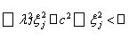
 , the operator Ax is defined on the whole space H. Its additivity and homogeneity are easy to verify, and its continuity follows easily from the inequality
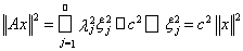

Each basis vector en is sent by the operator A into itself with coefficient λn: A en = λn en .
Example 5. On the segment [a, b] fix a continuous function α(x). In the space C[a,b] a linear operator of multiplication by α(x) is defined: 
 .
.
Example 6. Let X = Rn, Y = Rm. To every element x={ξ1, ξ2, ... , ξn} 
 Rn we assign, by means of the matrix (aij), i=1, 2, ... , m; j=1, 2, ... , n, an element y={
 1,
1,  2, ... , m} Rm , setting

 , i=1, 2, ... , m.
This defines an operator A: y = Ax, defined on Rn, with values in Rm. In this case one also says that the operator A is given by the matrix (aij), i = 1, 2, ... , m; j = 1, 2, ... , n. The linearity of the operator A was established in the course of linear algebra.
If 
 yk=Axk, y0=Ax0, then
 →
→ 
 for all j = 1, 2, ..., n, and hence,
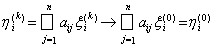
 , i = 1, 2, ... , m
But this means that yk = Axk 
 y0 = Ax0, and the operator A is continuous.
Example 7. Let X = Y = C[a, b]. For an arbitrary function 
 , let us set
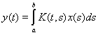
 (1)
(1)
where K(t, s) is a function continuous on the square 
 . Equality (1) defines an operator y = Ax, acting in C[a, b], which is called an integral operator . The additivity and homogeneity of the operator are practically obvious. For example:


Its continuity follows from the fact that convergence in the space C[a, b] is uniform convergence, under which one may pass to the limit under the integral sign. Hence if xn(t)→x0(t), then


Example 8. Let X = Y = L2[a, b]. Let us again consider the integral operator
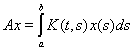
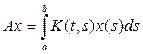
But now let us assume that the function K(t, s), called the kernel of the operator, is Lebesgue integrable on the square jointly in both variables:
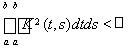

We show that the operator A acts in the space L2[a, b]. From the conditions k2 = 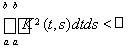
 and
and 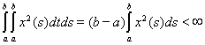
 it follows that K(t, s)x(s), as a function of both t and s, is integrable on . But then, by Fubini's theorem
is a measurable and integrable function, and Holder's inequality gives

 ,
,
i.e. that 
 . Taking the square root of the preceding expression, it can be written in the form
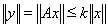
 . (2)
. (2)
The linearity of the operator A is obvious, and boundedness and continuity easily follow from inequality (2).
Example 9. Let X = Y = l2 and (aij), i, j = 1, 2, ..., be an infinite matrix such that
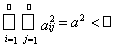
 . (3)
. (3)
Consider the operator A, defined by the following formal equality: for x ={ξi} 
 we set

 , i=1, 2, ... , and Ax = y = {
 }.
}.
First of all, the linearity of the operator A is obvious. Next, it follows from Hölder's inequality that the series 
 converges absolutely, since

 ,
,
i.e., the partial sums of the series 
 are bounded. Next,

 ,
,
and since this holds for any natural number n, then 
 , i.e.
 .
.
If we extract from the inequality
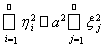

the square root, we obtain 
 . Hence, the operator A is bounded.
Lemma 2. A linear operator A, acting from X to Y, is bounded if it is bounded on at least one ball of the space X.
Proof. Since boundedness on an open ball implies boundedness on a closed ball with the same center and half the radius, we may at once assume that the operator is bounded on a closed ball. Let S[y, r] be the ball on which the operator A is bounded, i.e., ||Ax|| ≤ C for all x∈ S[y, r]. Take an arbitrary element z ∈X. From this element construct a new element z0 = y + rz/||z|| (or z = ||z||(z0 – y)/r). A direct computation shows that z0 ∈ S[y, r]. Hence ||Az0|| ≤ C. On the other hand, ||Az|| = ||z||/r(||A(z0 – y)||) ≤ ||z||/r(||Az0|| + ||Ay||) ≤ (2C/r)||z||, which proves the statement.
The most important property of a linear operator is its boundedness on S1 – the unit ball 
 of the space X. By Lemma 2 it implies the boundedness of the linear operator.
Let us set

 . (4)
. (4)
The number K0, defined by equality (4), is called the operator norm and denoted by ||A||. In the next section we shall show that this is indeed a norm. Thus, for any 


 .
.
Obviously, K0 = ||A|| is the smallest of the constants satisfying the inequality in the definition of boundedness, because if this were not so and there existed a number K' < K0 such that for all 
 , then for
 we would have
 , whence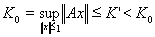
 , which is impossible.
Lemma 3. Let the linear operator A, acting from X to Y, be bounded on the ball S[y, r], i.e., ||Ax|| ≤ C for all x∈ S[y, r]. Then ||A|| ≤ 2C/r.
The statement was essentially established in the course of the proof of Lemma 2.
Computing the norms of specific operators is usually difficult, but it is often fairly easy to estimate the norm of an operator from above.
Example 10. Consider in the space C[a, b] the integral operator from Example 7. Let 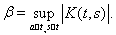
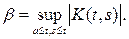 We have for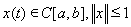
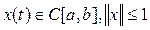 :
:
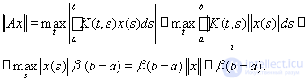
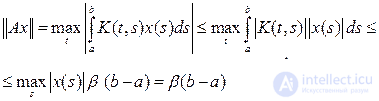
Hence 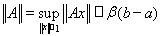
 , and we have estimated the norm of the integral operator in the space C[a, b].
Example 11. Consider in the same space C[a, b] the operator Bx = tx(t), called the operator of multiplication by the independent variable. For simplicity of computation we shall assume that 0 < a < b. For any function x(t)  C[a, b],
 we have

 (5)
(5)
Hence 
 . But if we take the function
 , then
 , and hence
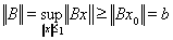
 (6)
(6)
From inequalities (5) and (6) it follows that ||B|| = b.
Example 12. The norm of the zero operator is obviously equal to zero. Conversely, if 
 , then it is easy to see that A=0.
Example 13. The norm of the identity operator I is equal to one, since ||Ix|| = ||x|| for any vector x.
Example 14. The norm of the similarity operator 
 is equal to
 .
.
Example 15. The norm of an operator of normal type in a Hilbert space
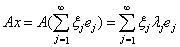
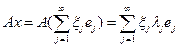
is equal to the exact upper bound of the numbers 
 . Indeed, if
 and
and 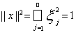
 , we have

whence 
 ; on the other hand
 , and the inequalities obtained prove our statement.

Comments