
Lecture
A bond graph is a graphical representation of a dynamic system, used when describing one or another physical (mechanical, electrical, hydraulic, pneumatic, economic, etc.) system, that reflects the process of energy redistribution within that system. It resembles a graph better known as a block diagram, or a signal-flow graph, and relies on the law of conservation of energy. The main difference from block diagrams or signal-flow graphs is that in a bond graph the edges are associated with a flow of energy, which can be directed in either direction, whereas block diagrams and signal-flow graphs assume a unidirectional flow of information. The edges in bond graphs are equipped with symbols specifying either an energy flow or an information flow.
Compared with other visual representation tools such as block diagrams, bond graphs have many advantages:
If the dynamics of the modeled system take place on different time scales, fast processes in real time can be treated as instantaneous phenomena using hybrid bond graphs.
In a bond graph a distinction is made between:
Exchanges between nodes are described by two parameters: flow and effort. Flow represents the change of a quantity per unit time: electric current I , volumetric flow rate of a liquid Qv , the velocity of an element v , etc. Effort represents the force by which the flow is driven: electrical voltage U , fluid pressure p , force F , etc. The product of flow and effort gives power, (measured in watts).
| Type of energy | Effort | Flow |
|---|---|---|
| mechanics, translation | force F , in newtons (N ) | linear velocity v , in meters per second (m/s ) |
| mechanics, rotation | torque C , in newton-meters (N⋅m ) | angular velocity ω , in radians per second (rad/s ) |
| electricity | voltage U , in volts (V ) | current I , in amperes (A ) |
| hydraulics | pressure p , in pascals (Pa ) | volumetric flow rate of a liquid Qv (in m3/s ) |
The edges of the graph — are half-arrows («harpoons»), whose barb elements are oriented downward or to the right: ⇁, ↽, ↾ ⇂. The direction of the arrow indicates the direction of power transfer, that is, power enters at the start of the arrow and leaves at its end. In the case of a measuring device (thermometer, tachometer, dynamometer, flow meter, manometer, voltmeter, ammeter, etc.) the energy flow is negligible, and a full arrow is used as the notation: →, ←, ↑ or ↓.
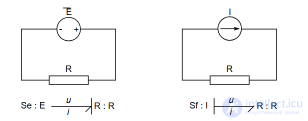
Bond graph for an electrical circuit with a resistance R and a voltage source (left) and a current source (right)
The laws governing the behavior at nodes often relate flow and effort. For example, for an electrical resistance, Ohm's law establishes the relationship between current and voltage :
U=R⋅I.
If the resistance is connected to a voltage source, then U is set at the source, and the resistance determines I . Conversely, if the resistance is connected to a current source, then I is set at it, and U is determined according to Ohm's law. Thus, there is causality. To indicate this on the diagram, a line is placed opposite the end of the arrow that defines the flow. This makes it possible to know the input value and the output value, obtained as a result of applying the law, that is, the value of the computed quantity: e=e(f) or f=f(e) .
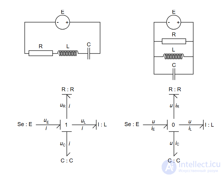
Bond graph for an RLC circuit in the case of series (left) and parallel (right) connections
A node can also represent a physical law rather than a particular element. A law that delivers the same effort e to several other nodes is called a 0-junction. A law that delivers the same flow f to several other nodes is called a 1-junction.
For the series connection in an RLC circuit there is only one branch. According to Kirchhoff's rule, all elements in such a circuit are given the same value of intensity (flow, current). This is a 1-junction. For the parallel connection in an RLC circuit, Kirchhoff's rule imposes the same voltage value on all elements; this is a 0-junction.
The directions of the arrows depend on the conventions chosen for the circuit.
Bond graphs characterize the transfer of power between the elements of a system, so they are ideally suited for modeling systems that connect several different domains of physics, such as, for example, electricity and mechanics. Before beginning to model, it is necessary to recall how the concept of power is introduced for each of these domains.
Power
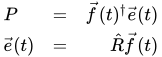
Power is defined as the product of flow and effort:

Momentum
A causal quantity defined by effort and related to it through integration:
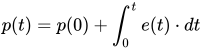
Displacement
A causal quantity defined by flow and related to it through integration:
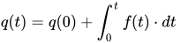
Many systems can be described using the terms used in bond graphs. These terms are presented in the table below.
Conventions for the table below:
 is the active power ;
 is a matrix object;
 is a vector object;
 is the Hermitian conjugate of x ; it is the complex conjugate of the transposed matrix x . If x — is a scalar, then the Hermitian conjugate coincides with the complex conjugate;
 — is the Euler notation for differentiation , where:Dtnf(t)={∫−∞tf(s)ds,n=−1f(t),n=0∂nf(t)∂tn,n>0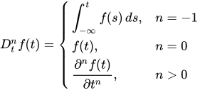
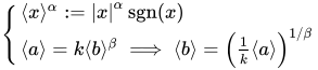
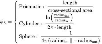
| Generalized flow | Generalized displacement | Generalized effort | Generalized momentum | Generalized power (in watts for power systems) | Generalized energy (in joules for power systems) | |
|---|---|---|---|---|---|---|
| Name |  |
 |
 |
p→(t) |
P=f→(t)†e→(t)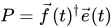 |
E=q→(t)†e→(t)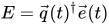 |
| Description | Time derivative of displacement | A quality related to static behaviour. | The energy per unit of displacement | Time integral of effort | Transformation of energy from one to another form. | Conserved quantity in closed systems |
| Elements | ||||||
| Name | Hyperance  hyperrigitance hyperrigitance |
ComplianceC rigitance rigitance |
Resistance  |
InertanceI (orL (orL ) ) |
AbrahanceA |
MagnanceM |
| Properties | Power dissipative element | charge storage element
(State variable: displacement) (Costate variable: effort) |
Power dissipative element | momentum storage element
(State variable: momentum) (Costate variable: flow) |
Power dissipative element | Power dissipative element |
| Quantitative behaviour | For one-dimensional systems (linear): 
For one-dimensional systems: Impedance: |
Potential energy for N-dimensional systems: 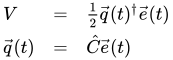
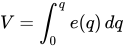
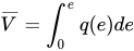
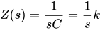
Potential energy:V=∫0qe(q)dq Potential coenergy :V¯=∫0eq(e)de For one-dimensional systems: Impedance:Z(s)=1sC=1sk |
For one-dimensional systems (linear) 
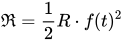
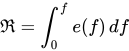
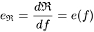
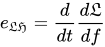
Power for one-dimensional non-linear resistances Rayleigh power:R=12R⋅f(t)2 Rayleigh power for non-linear resistances:R=∫0fe(f)df Rayleigh effort:eR=dRdf=e(f) For N -dimensional systems: ) For one-dimensional systems: Impedance: |
Kinetic energy for N -dimensional systems: 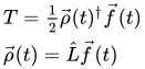
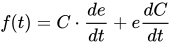
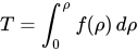
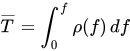
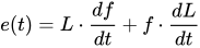
Kinetic energy:T=∫0ρf(ρ)dρ Kinetic coenergy:T¯=∫0fρ(f)df For one-dimensional systems:e(t)=L⋅dfdt+f⋅dLdt Impedance:Z(s)=sL |
For one-dimensional systems (linear): 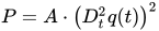
For one-dimensional systems:e(t)=A⋅γ[Dt3q(t)] ImpedanceZ(s)=s2A |
For one-dimensional systems (linear)P=A⋅(Dt3q(t))2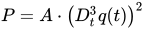
For one-dimensional systemse(t)=M⋅γ[Dt5q(t)] ImpedanceZ(s)=s4M |
| Generalized behaviour | Energy obtained from sources of active efforts: 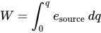
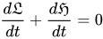
Lagrangian : Hamiltonian Hamiltonian effort Lagrangian effort: Passive effort: Power equation: Effort equation: Lagrangian equation: Hamiltonian equation: If
For linear elements |
| Flow-related variables | Dt6x : pounce / pop[m/s6] : pounce / pop[m/s6] |
Dt5x : flounce / crackle[m/s5] : flounce / crackle[m/s5] |
Dt4x : jounce / snap[m/s4] : jounce / snap[m/s4] |
Dt3x : jerk [m/s3] : jerk [m/s3] |
|---|---|---|---|---|
Dt2x : acceleration (x2t) [m/s2] : acceleration (x2t) [m/s2] |
Dt1x : velocity (xt) [m/s] : velocity (xt) [m/s] (flow) (flow) |
Dt0x : displacement(x) [m] : displacement(x) [m] (displacement) (displacement) |
Dt−1x : absement [m⋅s] : absement [m⋅s] |
|
Dt−2x : absity[m⋅s2] : absity[m⋅s2] |
Dt−3x : abseleration[m⋅s3] : abseleration[m⋅s3] |
Dt−4x : abserk[m⋅s4] : abserk[m⋅s4] |
||
| Effort-related variables | Dt1F : yank [N/s] : yank [N/s] |
Dt0F : force (Pxt) [N] : force (Pxt) [N] (effort) (effort) |
Dt−1F : linear momentum (Px2t) [kg⋅m/s] : linear momentum (Px2t) [kg⋅m/s] (momentum) (momentum) |
|
| Passive elements | ||||
| Compliance (C) | Resistance (R) | Inertance (I) | Abrahance (A) | Magnance (M) |
Spring〈Pxt〉=k〈x〉 wherek wherek is the spring stiffness is the spring stiffness |
Damper〈Pxt〉=b〈xt〉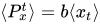 whereb whereb is the damper parameter is the damper parameter |
Mass〈Pxt〉=m〈x2t〉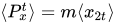 wherem wherem is the mass is the mass |
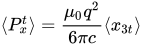
Abraham-Lorentz force
〈Pxt〉=μ0q26πc〈x3t〉
|
Magnetic radiation reaction force
〈Pqt〉=μ0q2R24πc3〈x5t〉
|
Cantilever beam〈F〉=3EI/L3〈x〉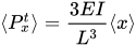
|
Resistance to cyclotron radiation
〈F〉=σTB2cμ0〈v〉
|
|||
| Prismatic float in a large pond
〈F〉=ρLgA〈x〉
|
Viscous friction〈F〉=b〈v〉whereb— is the viscous friction parameter |
|||
Elastic rod〈F〉=EA/L〈x〉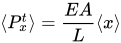
where
|
Inverse of kinetic mobility〈F〉=1μ〈v〉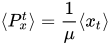 whereμ whereμ is the kinetic mobility is the kinetic mobility |
|||
| Newton's law of universal gravitation
〈F〉=GMm〈x〉−2
|
Interaction of geometry with air (e.g., air resistance)
〈F〉=12cρA〈v〉2
|
|||
| Coulomb's law
〈F〉=q1q24πε0〈x〉−2
|
Absquare [ clarification needed ] damper〈F〉=B〈v〉2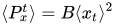 whereB whereB — is the parameter of the Absquare damper. — is the parameter of the Absquare damper. |
|||
| Casimir force
〈F〉=Aℏcπ2240〈x〉−4
|
dry friction
〈F〉=μFn〈v〉0
|
|||
| Biot–Savart law
〈F〉=μ0I1I2l2π〈x〉−1
|
||||
| A piston compresses fluid inside an adiabatic chamber.
F=AP0(1+xx0)−γ
|
| Flow-related variables | d3θ/dt3 angular jerk [rad/s3] angular jerk [rad/s3] |
d2θ/dt2 angular acceleration (θ2t) [rad/s2] angular acceleration (θ2t) [rad/s2]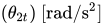 |
|---|---|---|
dθ/dt angular velocity (θt) [rad/s] angular velocity (θt) [rad/s] (flow) (flow) |
θ angular displacement (θ) [rad] angular displacement (θ) [rad] (displacement) (displacement) |
|
| Effort-related variables | dτ/dt : rotatum [V/rad] : rotatum [V/rad] |
τ : torque (θt) [J/rad] : torque (θt) [J/rad] (effort) (effort) |
∫τdt angular momentum (θ2t) [J⋅s/rad] angular momentum (θ2t) [J⋅s/rad]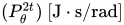 (momentum) (momentum) |
||
| Passive elements | ||
| Compliance (C) | Resistance (R) | Inertia (I) |
Inverse of the angular spring constant〈τ〉=k〈θ〉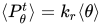 wherek wherek — is the angular spring constant. — is the angular spring constant. |
Angular damping〈τ〉=R〈θt〉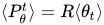 whereR— is the damping constant whereR— is the damping constant |
Mass moment of inertia
Type〈τ〉=J〈θ2t〉 whereJ |
| Torsion of a rod
〈τ〉=GJL〈θ〉
|
Governor (e.g., used in music boxes)〈τ〉=R〈θt〉2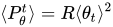 whereRis the governor constant whereRis the governor constant |
|
| Bending moment (cantilever)
〈τ〉=EJL〈θ〉
|
||
| Field of parallel forces
〈τ〉=〈F〉sin(α−θ)
|
| Flow-related variables | d2q/dt2 : rate of current change[A/s] : rate of current change[A/s] |
dq/dt electric current (qt) [A] electric current (qt) [A] (flow) (flow) |
q electric charge (q) [C] electric charge (q) [C] (displacement) (displacement) |
|
|---|---|---|---|---|
| Effort-related variables | dV/dt : voltage rate[V/s] : voltage rate[V/s] |
V : Voltage (qt) [V] : Voltage (qt) [V] (effort) (effort) |
∫Vdt : flux linkage (q2t) [V⋅s] or [Wb⋅turn] : flux linkage (q2t) [V⋅s] or [Wb⋅turn] (momentum) (momentum) |
|
| Elements | ||||
| Hyperactance (H) | Compliance (C) | Resistance (R) | Inertia (I) | Abrahance (A) |
| Frequency-dependent negative resistor (FDNR)
〈V〉=1H〈i〉 |
Linear capacitor
〈V〉=1εφL〈q〉
|
Linear resistor
〈V〉=ρφL(1+α(T−T0))〈i〉
|
Linear inductor (solenoid)
〈V〉=μ0N2AL〈q2t〉
|
Frequency-dependent negative conductance (FDNC)
Typeγ1⇔V=Rd2i/dt2[H⋅s] |
| Diode
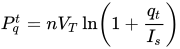
V=nVTln(1+iis)
|
Toroid
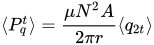
〈V〉=μN2A2πr〈q2t〉
|
|||
| Intra-gyrator | Inter-gyrator | |||
| Compliant gyrator | Resistive gyrator | Inertial gyrator | ||
| Hall effect device
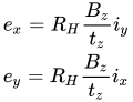
ex=RHBz/tz⋅iy ey=RHBz/tz⋅ix
|
Induction motor
er1=Mcos(θ)dφs1/dt+φs1d[Mcos(θ)]/dt es1=Mcos(θ)dφr1/dt+φr1d[Mcos(θ)]/dt
|
DC motor
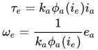
τe=kaφa(if)ia ωe=1kaφa(if)ea
|
Faraday vibration generator
F=Bli V=Blv
|
|
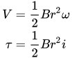
| Faraday disk
V=12Br2ω τ=12Br2i
|
||||
| Intra-transformer | Inter-transformer | |||
| Electrical transformer (AC signals only)
V2=N2N1V1 φ2=N1N2φ1 |
| Flow-related variables | dV/dtvolumetric flow rate (Vt) [m3/s] (flow) (flow) |
V: volume (V) [m3] (displacement) (displacement) |
|---|---|---|
| Effort-related variables | P : pressure (PVt) [Pa] : pressure (PVt) [Pa] (effort) (effort) |
∫Pdt : fluid momentum(PV2t) [Pa⋅s] : fluid momentum(PV2t) [Pa⋅s]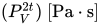 (momentum) (momentum) |
| Elements | ||
| Compliance (C) | Resistance (R) | Inertia (I) |
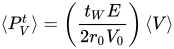
| Pipe elasticity
〈P〉=(tVE2r0V0)〈V〉
|
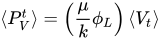
Darcy sponge
〈P〉=(μkφL)〈Vt〉
|
Fluid inertia in pipes
〈P〉=(ρφL)〈V2t〉
|
| Compressible fluid (approximation)
〈P〉=(BV0)〈V〉=(ρ0c2V0)⏟AcousticApproximation〈V〉
|
продолжение следует...
Часть 1 Bond Graph
Часть 2 Tetrahedron of State - Bond Graph
Часть 3 State equations - Bond Graph

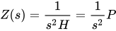
 (this is the effort applied by the element):P=e(f)f














 is the coenergy
  is the energy,
 is the state variable and
 is the costate variable,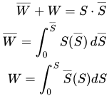
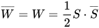
 where
where is the permeability
 is the electric charge
 — is the speed of light.
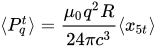 where
where Young's modulus
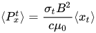 where
where : Thomson cross section
 where
where : liquid density
 : gravitational acceleration
 where
where : gravitational constant
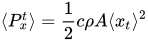 where
where : fluid density
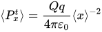 where
where permittivity
 : charge of body 1
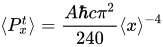 where
where : reduced Planck constant
 where
where : normal force
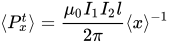 where
where : current in wire 1
 : current in wire 2
 length of the wires
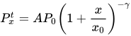 where
where initial internal pressure
 : initial piston position
 adiabatic index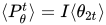
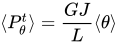 where
where : polar moment of area
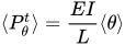 where
where where
where : angle (positive counterclockwise) between the polar axis and the force field
 : current tilt angle of the object (e.g., a pendulum)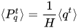
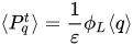 where
where : permittivity
 : geometry factor
 where
where : current temperature
 reference temperature
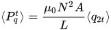 where
where : number of turns
 where
where ideality factor
 : thermal voltage
 leakage current
 where
where toroid radius relative to the centerline
 where
where Hall coefficient
 : vertical magnetic flux density
 : vertical thickness
 where
where : rotor bar voltage
 : stator bar voltage
 flux through the stator bar
 flux through the rotor bar
 where
where electromagnetic torque
 : shaft angular velocity
 : field current
 armature current
 where
where : force
 : rod voltage
 where
where
 where
where nominal pipe radius
 : pipe volume (unstressed)
 : wall thickness
 where
where where
where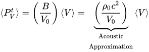 where
where

Comments