
Lecture
By the nature of control:
By the nature of action:
By the degree of use of information about the state of the controlled object:
By the degree of use of information about the parameters and structure of the controlled object:
By the degree of coordinate transformation in the ACS:
By the type of mathematical model of coordinate transformation:
By the type of control actions:
By the degree of human participation:
By the law of change of the output variable:
By the number of controlled and regulated variables:
By the degree of self-tuning, adaptation, optimization and intelligence:
By the effect of the sensing (measuring) element on the regulating unit:
IACS — are systems that allow learning, adaptation or tuning to be carried out by storing and analyzing information about the behavior of the object, its control system and external actions. A characteristic feature of these systems is the presence of a database, an inference engine, an explanation subsystem, etc.
Knowledge base — formalized rules in the form of logical formulas, tables, etc. An ICS is used to control poorly formalized or complex technical objects.
An ICS class corresponds to the following features:
If an ICS satisfies all 5 features, then it is intelligent in the «large» sense, otherwise in the «small» sense.
By the type of mathematical description (equations of dynamics and statics), automatic control systems (ACS) are divided into linear and nonlinear systems (ACS or ARS).
Each “subclass” (linear and nonlinear) is further divided into a number of “subclasses”. For example, linear ACS (ARS) differ by the type of mathematical description.
Since this semester will consider the dynamic properties of only linear automatic control (regulation) systems, below is a classification by type of mathematical description for linear ACS (ARS):
1) Linear automatic control systems, described in «input-output» variables by ordinary differential equations (ODEs) with constant coefficients:

where x(t) – input action; y(t) – output action (controlled quantity).
If an operator («compact») form of writing the linear ODE is used, equation (1.4.1) can be represented as follows:

where, p = d/dt — differentiation operator; L(p), N(p) — corresponding linear differential operators, which are equal to:

2) Linear automatic control systems, described by linear ordinary differential equations (ODEs) with variable (time-varying) coefficients:

In general, such systems can also be classified as nonlinear ACS (ARS).
3) Linear automatic control systems, described by linear difference equations:

where f(…) – a linear function of the arguments; k = 1, 2, 3… — integers; Δt – the sampling interval (quantization interval).
Equation (1.4.4) can be represented in «compact» form:

Usually such a description of linear ACS (ARS) is used in digital control systems (using a computer).
4) Linear automatic control systems with time delay:

where L(p), N(p) — linear differential operators; τ — the delay time or delay constant.
If the operators L(p) and N(p) degenerate (L(p) = 1; N(p) = 1), then equation (1.4.6) corresponds to the mathematical description of the dynamics of an ideal time-delay element:
y(t)=x(t−τ);
and a graphical illustration of its properties is shown in fig. 1.4.1
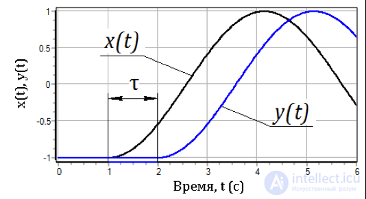
Fig. 1.4.1 — Input and output graphs of an ideal time-delay element
5) Linear automatic control systems, described by linear differential equations in partial derivatives. Such ACS are often called distributed control systems. ==> An «abstract» example of such a description:

The system of equations (1.4.7) describes the dynamics of a linearly distributed ACS, i.e. the controlled quantity depends not only on time, but also on one spatial coordinate.
If the control system represents a «spatial» object, then ==>

where y(t,r→) depends on time and the spatial coordinates determined by the radius vector r→
6) ACS described by systems of ODEs, or by systems of difference equations, or by systems of partial differential equations ==> and so on…
A similar classification can be proposed for nonlinear ACS (ARS)…
For linear systems the following requirements hold:
The static characteristic is defined as the dependence of the output on the magnitude of the input action in steady state (when all transient processes have decayed).
For systems described by linear ordinary differential equations with constant coefficients, the static characteristic is obtained from the dynamics equation (1.4.1) by setting all non-stationary terms to zero ==>

Fig. 1.4.2 shows examples of linear and nonlinear static characteristics of automatic control (regulation) systems.
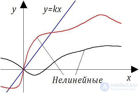
Fig. 1.4.2 — Examples of static linear and nonlinear characteristics
Nonlinearity of the terms containing time derivatives in the dynamics equations can arise from the use of nonlinear mathematical operations ( 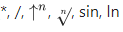 etc.). For example, considering the dynamics equation of some «abstract» ACS

note that in this equation, for a linear static characteristic (y=kd⋅x), the second and third terms (dynamic terms) on the left-hand side of the equation are nonlinear, and therefore the ACS described by such an equation is nonlinear in the dynamic sense.
By the nature of the transmitted signals, automatic control (or regulation) systems are divided into:
A system of continuous action is an ACS in which, in each of its elements, a continuous change of the input signal in time corresponds to a continuous change of the output signal, while the law of change of the output signal can be arbitrary. For an ACS to be continuous, it is necessary that the static characteristics of all elements be continuous.
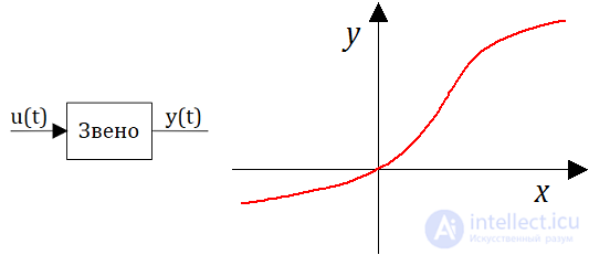
Fig. 1.4.3 — Example of a continuous system
A system of relay action is an ACS in which, in at least one element, with a continuous change of the input quantity, the output quantity at certain moments of the control process changes “in a jump” depending on the value of the input signal. The static characteristic of such an element has points of discontinuity or a break with a discontinuity.
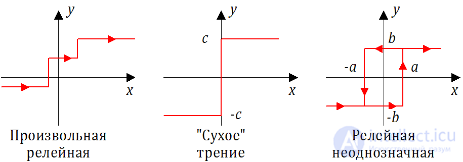
Fig. 1.4.4 — Examples of relay static characteristics
A system of discrete action is a system in which, in at least one element, with a continuous change of the input quantity, the output quantity has the form of separate pulses appearing after a certain interval of time.
An element that converts a continuous signal into a discrete signal is called a pulse element. This type of transmitted signal occurs in an ACS with a computer or a controller.
The following methods (algorithms) for converting a continuous input signal into a pulse output signal are most often implemented:
Fig. 1.4.5 shows a graphical illustration of the pulse-amplitude modulation (PAM) algorithm. The upper part of the figure shows the time dependence x(t) — the signal at the input of the pulse element. The output signal of the pulse block (element) y(t) – a sequence of rectangular pulses appearing with a constant sampling period Δt (see the lower part of the figure). The pulse duration is the same and equal to Δ. The amplitude of the pulse at the output of the block is proportional to the corresponding value of the continuous signal x(t) at the input of this block.
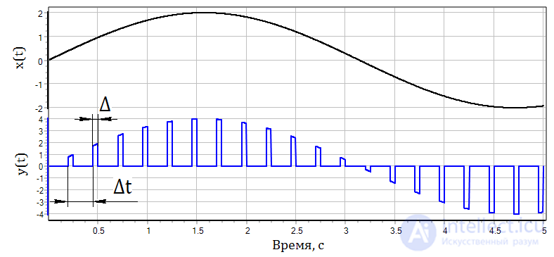
Fig. 1.4.5 — Implementation of pulse-amplitude modulation
This pulse modulation method was quite widespread in the electronic measuring equipment of control and protection systems (CPS) of nuclear power plants (NPP) in the 1970s…1980s.
Fig. 1.4.6 shows a graphical illustration of the pulse-width modulation (PWM) algorithm. The upper part of fig. 1.14 shows the time dependence x(t) – the signal at the input of the pulse element. The output signal of the pulse block (element) y(t) – a sequence of rectangular pulses appearing with a constant sampling period Δt (see the lower part of fig. 1.14). The amplitude of all pulses is the same. The pulse duration Δt at the output of the block is proportional to the corresponding value of the continuous signal x(t) at the input of the pulse block.
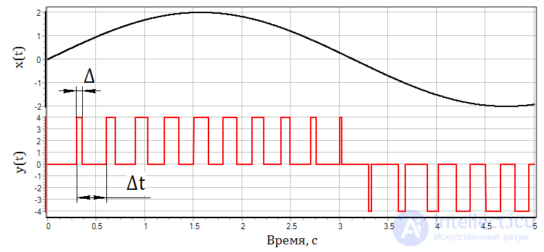
Fig. 1.4.6 — Implementation of pulse-width modulation
This pulse modulation method is currently the most widespread in the electronic measuring equipment of control and protection systems (CPS) of nuclear power plants (NPP) and the ACS of other technical systems.
To conclude this subsection, it should be noted that if the characteristic time constants in other elements of the ACS (ARS) are substantially greater than Δt (by orders of magnitude), then the pulse system can be considered a continuous automatic control system (when using either PAM or PWM).
By the nature of the control processes, automatic control systems are divided into the following types:
The stochastic output signal is characterized by:
The stochastic nature of the control process is usually observed in substantially nonlinear ARS both from the standpoint of the static characteristic and from the standpoint (even to a greater degree) of the nonlinearity of the dynamic terms in the dynamics equations.
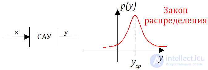
Fig. 1.4.7 — Distribution of the output quantity of a stochastic ACS
In addition to the main classifications of control systems given above, there are other classifications. For example, a classification can be based on the method of control and on the interaction with the external environment and the ability of the ACS to adapt to changes in environmental parameters. Systems are divided into two large classes:
1) Ordinary (non-self-tuning) control systems without adaptation; these systems are classified as simple, not changing their structure during the control process. They are the most developed and widely used. Ordinary control systems are divided into three subclasses: open-loop, closed-loop and combined control systems.
2) Self-tuning (adaptive) control systems. In these systems, when external conditions or the characteristics of the controlled object change, an automatic (not predetermined) change of the parameters of the controller occurs, due to a change in the coefficients of the control system, the structure of the control system, or even the introduction of new elements.
Another example of classification: by hierarchical level (single-level, two-level, multi-level).

Comments