
Lecture
Это продолжение увлекательной статьи про бондграф.
...
data-auto-open loading="lazy" alt="Bond Graph" >: gas density at reference pressure
 speed of sound
〈P〉=(ρ2Cd2A02)〈Vt〉2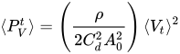
 discharge coefficient
 : fluid density
 : minimum flow area
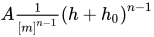 :
:
PVt=ρgh0[(1+nVA1[m]n−1h0n)1/n−1]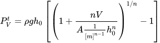 where
where
 height above the ground
 inlet height: fluid density
 : curve scaling (area dimension)
 : dimensional correction
 : curve parameter
 : gravitational acceleration
 (prismatic body):PVt=ρgAV
 (diode case):PVt=ρgh0(eVA[m]−1)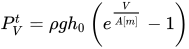
〈P〉=(8μLπR4)〈Vt〉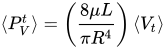 where
where
 dynamic viscosity
 : pipe length
 pipe radius
〈P〉=k〈Vt〉−1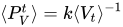 wherek
 is the chamber constant
〈P〉=at〈Vt〉74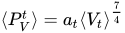 whereat
 is an empirical parameter
PVt=−BlnV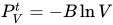 whereB
 — is the bulk modulus.
〈P〉=ρ2(Avne2‖−Av2)〈Vt〉2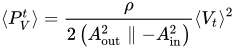 where
where
: fluid density : exit area
 : entry area
PBt=PB,0t(1−BB0)−γ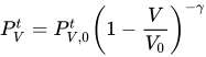 where
where
 : reference pressure
 : reference volume
 Poisson’s ratio
PBt=kln(1+BtBt,0)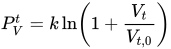 where
where
empirical constant : reverse absolute displacement flow
| Flow-related variables | Dt0φ magnetic flux (φ) [Wb] magnetic flux (φ) [Wb] (displacement) (displacement) |
|
|---|---|---|
| Effort-related variables | Dt0F magnetomotive force (Φ) [A⋅turn] magnetomotive force (Φ) [A⋅turn]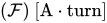 (momentum) (momentum) |
|
| Elements | ||
| Compliance (C) | Resistance (R) | Inertia (I) |
Permeance (P ) )
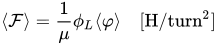
〈Φ〉=1μϕL〈φ〉[H/turn2]
|
Magnetic complex impedance (ZM ) )
Φ=ZMφt[turn2/Ω] |
Complex magnetic inductance (LM ) )
Φ=LMφ2t[turn2Φ] |
| Flow-related variables | Dt0Ig : gravitational current loop(Ig=2εgvorbita3) [kg/s] : gravitational current loop(Ig=2εgvorbita3) [kg/s] (flow) (flow) |
Dt−1Ig gravitational charge(M) [kg] gravitational charge(M) [kg] (displacement) (displacement) |
|---|---|---|
| Effort-related variables | Dt0Bg : gravitational voltage(Bg=12vorbita4c2) [m2/s2] : gravitational voltage(Bg=12vorbita4c2) [m2/s2]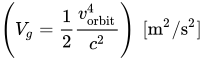 (effort) (effort) |
Dt−1Bg gravitational momentum(ϕg=πvorbita3pc2) [m2/s] gravitational momentum(ϕg=πvorbita3pc2) [m2/s]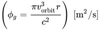 (momentum) (momentum) |
| Elements | ||
| Compliance (C) | Resistance (R) | Inertia (I) |
| Gravitational capacitance
Typeγ1⟺Mg=CBg[kg/m2] Cg=2c2p2GM |
Gravitational orbital resistance
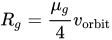
Typeγ1⟺Bg=RgIg[m2/kg⋅s] Rg=μg4vorbita |
Gravitational inductance
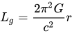
Typeγ1⟺ϕg=IIg[m2/kg⋅s2] Lg=2π2Gc2p |
| Flow-related variables | Dt0J. : current density (J.) [A/m2] : current density (J.) [A/m2] (flow) (flow) |
Dt−1J. : electric displacement field (D) [C/m2] : electric displacement field (D) [C/m2] (displacement) (displacement) |
|---|---|---|
| Effort-related variables | Dt0E : electric field (E) [V/m] : electric field (E) [V/m] (effort) (effort) |
Dt−1E : magnetic vector potential(A) [V⋅s/m] : magnetic vector potential(A) [V⋅s/m]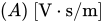 (momentum) (momentum) |
| Elements | ||
| Compliance (C) | Resistance (R) | Inertia of volumetric power density (IB ) ) |
| Electric permittivity
Typeγ1⟺D=ϵ0E[F/m] |
Electrical resistivity
Typeγ1⟺E=ρJ.[Ωm] |
Magnetic permeability μ0 [H/m] |
| Flow-related variables | Dt0B : magnetic flux density(B) [T] or [Wb/m2] : magnetic flux density(B) [T] or [Wb/m2] (displacement) (displacement) |
|
|---|---|---|
| Effort-related variables | Dt0H : magnetic field strength(H) [A⋅turn/m] : magnetic field strength(H) [A⋅turn/m] (effort) (effort) |
|
| Elements | ||
| Compliance (C) | Resistance (R) | Inertia of volumetric power density (IB) |
| Magnetic permeability for magnetic circuits
Type γ1⟺B=μH[H/(m⋅turn2)] |
| Flow-related variables | Dt0J.g : mass flow(J.g) [kg/m2s] : mass flow(J.g) [kg/m2s]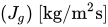 (flow) (flow) |
Dt−1J.g : accumulated mass flow(Dg) [kg/m2] : accumulated mass flow(Dg) [kg/m2]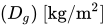 (displacement) (displacement) |
|---|---|---|
| Effort-related variables | Dt0g : gravitational acceleration (g) [m/s2] : gravitational acceleration (g) [m/s2] (effort) (effort) |
|
| Elements | ||
| Compliance (C) | Resistance (R) | Inertia of volumetric power density (IB) |
| Gravitational dielectric permittivity
Typeγ1⟺Dg=ϵgg[kg⋅s2/m3] εg=14πG |
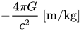
Gravitational permeability[m/kg] IB=μg=4πGc2 IB=μg=4πGc2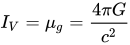 |
| Flow-related variables | Dt0Bg gravitomagnetic field(Bg=ωorbita(vorbitac)2) [Hz] gravitomagnetic field(Bg=ωorbita(vorbitac)2) [Hz]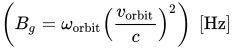 (displacement) (displacement) |
|
|---|---|---|
| Effort-related variables | Dt0Hg : gravitomagnetic field strength(Hg) [Pa⋅s] : gravitomagnetic field strength(Hg) [Pa⋅s] (effort) (effort) |
|
| Elements | ||
| Compliance (C) | Resistance (R) | Inertia of volumetric power density (IB) |
| Gravitational permeability
−4πGc2 [m/kg] |
| Flow-related variables | Dt1B heating rate(ψt) [W] heating rate(ψt) [W] (flow) (flow) |
Dt0B : total heat(ψ) [J.] : total heat(ψ) [J.] (displacement) (displacement) |
|---|---|---|
| Effort-related variables | Dt0T : temperature(T) [K] : temperature(T) [K] (Effort) (Effort) |
|
| Elements | ||
| Compliance (C) | Resistance (R) | Inertia (I) |
| Isobaric heating
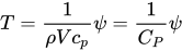
T=1ρBcpψ=1CPψ
|
Conduction resistance
T=1kϕLψt
|
|
| Isochoric heat
T=1CBψ |
Convection resistance
T=1hAψt
|
|
| Isothermal heat
T=1nRln(BfBi)ψ
|
Stefan-Boltzmann law
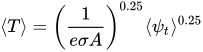
〈T〉=(1eσA)0,25〈ψt〉0,25
|
| Flow-related variables | Dt1ε strain rate(ε˙) [Hz] strain rate(ε˙) [Hz] (flow) (flow) |
Dt0ε : strain(ε) : strain(ε)  (displacement) (displacement) |
|---|---|---|
| Effort-related variables | Dt0σ : stress(σ) [Pa] : stress(σ) [Pa] (effort) (effort) |
|
| Elements | ||
| Compliance (C) | Resistance (R) | Inertia of volumetric power density (IB) |
| Reciprocal of stiffness
Typeγ1⟺ε=Cσ[Pa−1] C=1K |
Viscosity
Typeγ1⟺σ=Rε˙[Pa⋅s] |
Inertial force, determined by power density: material density.
ρ [kg/m3] |
Other systems:
Tetrahedron of state
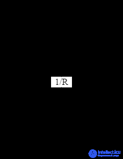
The tetrahedron of state is a tetrahedron that graphically displays the transformation between effort and flow. The attached image shows the tetrahedron in its generalized form. The tetrahedron can be modified depending on the energy domain.
Using the tetrahedron of state, the mathematical relationship between any variables on the tetrahedron can be found. This is done by following the arrows on the diagram and multiplying any constants along the way. For example, if you want to find the relationship between generalized flow and generalized displacement, you would start with f ( t ) , and then integrate it to get q ( t ) . More examples of equations can be seen below.
Relationship between generalized displacement and generalized flow.
q(t)=∫f(t)dt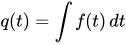
Relationship between the generalized flow state and generalized effort.
f(t)=1R⋅e(t)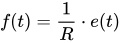
Relationship between generalized flow and generalized momentum.
f(t)=1I⋅p(t)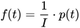
Relationship between general momentum and general effort.
p(t)=∫e(t)dt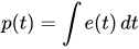
Relationship between generalized flow and generalized effort, involving constant C.
e(t)=1C∫f(t)dt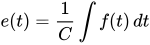
All mathematical relationships remain unchanged when moving between energy domains; only the symbols change. This can be seen in the following examples.
Relationship between displacement and velocity.
x(t)=∫v(t)dt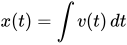
Relationship between current and voltage, also known as Ohm’s law .
I(t)=1RV(t)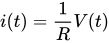
Relationship between force and displacement, also known as Hooke’s law . The negative sign in this equation is omitted, since the sign is accounted for by the direction of the arrow on the bond graph.
F(t)=kx(t)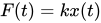
For energy systems, the formula for the resonant frequency is as follows:ω=1LC
For systems with high specific power, the formula for the resonant wave speed is as follows:c=1LC
If a motor is connected to a wheel through a shaft, power is transmitted in the rotational-mechanical domain, meaning effort and flow represent torque (τ) and angular velocity (ω), respectively. A word bond graph — is the first step toward a bond graph, in which words define the components. As a word bond graph, this system would look as follows:motor−−−−−ωτwheel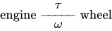 A half arrow is used to denote signs, so if the motor does work when τ and ω are positive, then the diagram would look as follows:motor−−−⇁ωτwheel
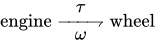 This system can also be represented in a more general way. This involves replacing the words with symbols denoting the same elements. These symbols are based on the generalized form, as explained above. Since the motor generates torque on the wheel, it will be represented as an effort source for the system. The wheel can be represented as a resistance to the system. In addition, the symbols for torque and angular velocity are omitted and replaced with the generalized symbols for effort and flow. Although this is not necessary in this example, bonds are usually numbered to avoid confusion in the equations. A simplified diagram is shown below.

Since effort always exceeds flow along a bond, the effort and flow symbols can also be omitted entirely without losing any important information. However, the bond number should not be omitted. An example can be seen below.

The bond number will become important later when converting the bond graph into state-space equations.
Suppose an element has the following behavior:e(t)=αg(q(t)) whereg(x)
 is a universal function (it can even differentiate/integrate its inputs) andα
 — is the element constant. Now suppose that a 1-junction has many elements of this type. Then the total effort at the junction equals:e
Suppose an element has the following behavior:e(t)=g(αq(t)) whereg(x)is a universal function (it can even differentiate/integrate its inputs) andα— is the element constant. Now suppose that a 0-junction has many elements of this type. Then the following holds:

One-port elements — are elements in the bond graph that can have only one port.
Sources — are elements that represent inputs to the system. They either input effort or supply flow into the system. They are denoted by the capital letter «S», with «e» or «f» — lowercase letters denoting effort or flow, respectively. Sources always have an arrow pointing away from the element. Examples of sources include: motors (an effort source, torque), voltage sources (an effort source), and current sources (a flow source).
 where J denotes a junction.
Sinks are elements that represent the output data of the system. They are depicted the same way as sources, but the arrow points into the element rather than away from it.

Inertia elements are denoted by the capital letter «I» and always pass energy through themselves. Inertia elements are elements that store energy. Most often these are mass in mechanical systems and inductors in electrical systems.

Resistive elements are denoted by the capital letter «R» and always pass electric current through themselves. Resistive elements are elements that dissipate energy. Most often these are dampers in mechanical systems and resistors in electrical systems.

Compliant elements are denoted by the capital letter «C» and always pass electric current through themselves. Compliant elements are elements that store potential energy. Most often these are springs in mechanical systems and capacitors in electrical systems.
J.−−−⇀ C
These elements have two ports. They are used to convert power between systems or within them. When converting power from one port to another, there is no power loss during transmission. Each element has a specified constant. This constant is called the transformer constant or the gyrator constant, depending on which element is used. As a rule, these constants are displayed as a coefficient next to the element.
The transformer establishes a relationship between the incoming and outgoing flow and the incoming and outgoing effort. Examples include an ideal electrical transformer or a lever.
Denoted−−−⇀1 TF −−−⇀2 r:1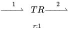 where r denotes the transformer modulus. This means that...f1r=f2
 and e2r=e1
A gyrator uses the relationship between the incoming and outgoing flow of energy and the incoming flow of energy. An example of a gyrator is a DC motor, which converts voltage (electrical effort) into angular velocity (angular mechanical flow).
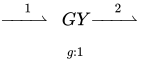 this means that e2=gf1
 and e1=gf2.
Unlike other elements, junctions can have any number of input or output ports. Junctions distribute power among their ports. There are two different types of junctions: the 0-junction and the 1-junction, which differ only in the way effort and flow are transmitted. Identical junctions connected in series can be merged, but different junctions connected in series cannot.
Zero junctions behave in such a way that all effort values (and their time integral/derivative) are equal across all connections, but the sum of the incoming flow values equals the sum of the outgoing flow values, or, equivalently, the sum of all flows is zero. In an electrical circuit, a zero junction is a node representing the voltage shared by all the components at that node. In a mechanical circuit, a zero junction is a connection between components representing the force shared by all the components connected to it.
all e' are equal
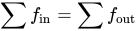
An example is shown below.
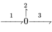
The resulting equations:e1=e2=e3 f1=f2+f3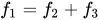
1-junctions behave oppositely to 0-junctions. In 1-junctions, all flow values (and their time integral/derivative) are equal across all connections, but the sum of the input effort values equals the sum of the output effort values, or, equivalently, the sum of all efforts is zero. In an electrical circuit, a 1-junction represents a series connection of components. In a mechanical circuit, a 1-junction represents the velocity shared by all the components connected to it.
all f' are equal ∑ein=∑eout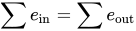
An example is shown below.
−−−⇁11↾2−−−⇁3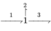
The resulting equations:f1=f2=f3

Bond graphs contain the concept of causality, which indicates which side of a bond determines the instantaneous effort and which determines the instantaneous flow. When formulating the dynamic equations describing a system, causality determines, for each modeling element, which variable is dependent and which is independent. Graphically propagating causality from one modeling element to another simplifies the analysis of large-scale models. Completing the causality assignment in a bond graph model makes it possible to detect modeling situations in which an algebraic loop exists; that is, a situation in which a variable is defined recursively as a function of itself.
As an example of causality, consider a capacitor connected in series with a battery. It is physically impossible to charge a capacitor instantaneously, so any component connected in parallel with the capacitor will necessarily have the same voltage (the involved variable) as the capacitor. Similarly, an inductor cannot instantaneously change its magnetic flux, so any component connected in series with the inductor will necessarily have the same flow as the inductor. Because capacitors and inductors are passive devices, they cannot maintain their respective voltage and flow indefinitely — the components to which they are connected will affect their respective voltage and flow, but only indirectly, by affecting their current and voltage respectively.
Note: Causality is symmetric. When one side «causes» the effort, the other side «causes» the flow.
In the graphical notation of bonds, a causal stroke can be added to one end of a power bond, indicating that this side determines the flow . Consequently, the side opposite the causal stroke controls effort .
Flow sources (Sf ) determine the flow, so they carry the causal stroke:Sf|−−−⇀
 Effort sources (Se
 ) determine the effort, so the causal stroke is at the other end:Se−−−⇀|
Consider a motor with constant torque driving a wheel, i.e., an effort source (SeThis will be depicted as follows:motorSe−−−⇀|ωτwheel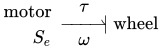
Symmetrically, the side with causal motion (in this case, the wheel) determines the direction of flow for the bond.
Causality leads to compatibility constraints. Obviously, only one end of a power bond can determine effort, and therefore only one end of the bond (the other end) can carry the causal stroke. Furthermore, the two passive components with time-dependent behavior,I andC
andC , can have only one kind of causality:Ithe component determines the flow;Cthe component determines the effort. Thus, from the junction point,J.
 the preferred causal orientation is as follows:J.−−−⇀|I and J.|−−−⇀C
The reason this method is preferred for these elements can be further analyzed by considering the equations they yield, shown by the state tetrahedron.

The resulting equations include the integral of the independent power variable. This is preferable to the result obtained when the causality is reversed, which leads to a derivative. The equations are given below.

In a bond graph, it is possible for the causal stroke on one of these elements to be placed in a less preferred way. In such a case, the bond is said to have a «causal conflict». The consequences of a causal conflict are only apparent when writing out the graph's state equations. This is explained in more detail in the relevant section.
A resistor does not exhibit time-dependent behavior: applying a voltage produces an instantaneous current, or applying a current produces an instantaneous voltage, so a resistor can be placed at either end of the causal bond: 
Transformers are passive, they neither dissipate nor store energy, so causality passes through them:−−−−−|TF−−−−−|or|−−−−−TF|−−−−−
A gyrator converts flow into effort and effort into flow, so if flow occurs on one side, effort occurs on the other side, and vice versa:|−−−−−GY−−−−−|or−−−−−|GY|−−−−−
In a zero junction, the efforts are equal; in a one junction, the flows are equal. Thus, when causality is assigned, only one bond can impose effort at a zero junction, and only one bond can impose flow at a one junction. Consequently, if the causality of one bond at the junction is known, the causality of the rest is also known. This one bond is called the «strong bond».strong bond→⊣0⊥⊤⊣andstrong bond→⊢1⊤⊥⊢ In short, 0-junctions must have exactly one causal stroke, and 1-junctions must have all causal strokes except one.
To determine causality in a bond graph, certain steps must be performed. These steps are as follows:
A step-by-step description of the process is given below.Sf−−−⇀0−−−⇀TF−−−⇀0−−−⇀C5⇃r:1⇃C2R6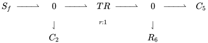
The first step is to assign causality between sources, for which only one source exists. The result is the graph shown below.Sf|−−−⇀0−−−⇀TF−−−⇀0−−−⇀C5⇃r:1⇃C2R6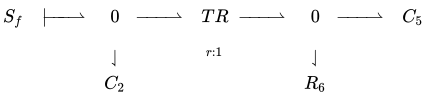
The next step is to determine the preferred causality for the C bonds.Sf|−−−⇀0−−−⇀TF−−−⇀0|−−−⇀C5⇃¯r:1⇃C2R6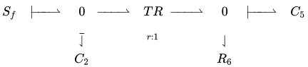
Next, apply causality to the zero and one junctions, transformers, and gyrators.Sf|−−−⇀0|−−−⇀TF|−−−⇀0|−−−⇀C5⇃¯r:1⇃_C2R6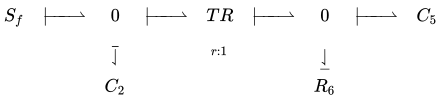
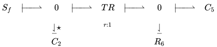
However, there is a problem with the zero junction on the left. The zero junction has two bonds imposing effort, whereas the zero junction needs only one. This happened becauseC2 is required to be in its preferred causality. The only way to fix this is to reverse this causal stroke. This leads to a causal conflict; the corrected version of the graph is shown below.⋆
 reflecting the causal conflict.
One of the main advantages of using bond graphs is that once the bond graph has been obtained, the original energy domain no longer matters. Below are some steps that must be followed when converting from an energy domain to a bond graph.
A step-by-step solution of an electromagnetic problem as a bond graph looks as follows:
These steps are illustrated more clearly in the examples below.
The sequence of steps for solving a linear mechanics problem as a bond graph is as follows:
These steps are illustrated more clearly in the examples below.
The simplification stage is the same regardless of whether the system is electromagnetic or linear-mechanical. The steps are as follows:
These steps are illustrated more clearly in the examples below.
Parallel power transmission is when power is transmitted in parallel in a bond graph. An example of parallel power transmission is shown below.
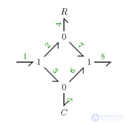
The parallel power equation can be simplified by recalling the effort–flow relationship for 0- and 1-junctions. To solve the parallel power equation, all the junction equations must first be written out. For the example given, the equations are shown below. (Note the numeric value represented by the effort/flow variable.)f1=f2=f3e2=e4=e7e1=e2+e3f2=f4+f7e3=e5=e6f7=f6=f8f3=f5+f6e7+e6=e8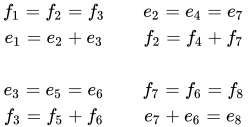
By manipulating these equations, you can arrange them in such a way as to find an equivalent set of 0- and 1-junctions to describe the parallel effort bond.
For example, becausee3=e6 ande2=e7
 you can substitute the variables in the equatione1=e2+e3
 which results ine1=e6+e7
 and sincee6+e7=e8
 we now know thate1=e8
 This relationship between two effort variables being equal to zero can be explained by a 0-junction. Manipulating the other equations, it can be found thatf4=f5
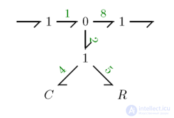
 This describes the relationship of a 1-junction. Once you have identified the necessary relationships, you can redraw the parallel power section with the new junctions. The result for the example shown is presented below.
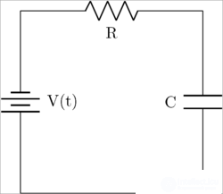
A simple electrical circuit consisting of a voltage source, a resistor, and a capacitor connected in series.
The first step is to draw 0-junctions at all nodes:0000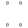
The next step is to add all the elements acting at their own junction points:R|0−1−0||Se−11−C||0_−−−0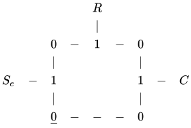
The next step is to choose the ground. The ground is simply a 0-junction that is considered to have no voltage. In this case, the bottom left 0-junction, underlined above, will be chosen as the ground. The next step is to draw all the arrows for the bond graph. The arrows at the junctions must point toward the ground (following a path similar to the current). For the resistance, inertia, and compliance elements, the arrows always point toward those elements. The result of drawing the arrows is shown below, where the 0-junction is marked with an asterisk as the ground.
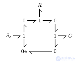
Now that we have the bond graph, we can begin the process of simplifying it. The first step is to remove all the ground nodes. Both lower 0-junctions can be removed, since they are both grounded. The result is shown below.
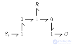
Next, junctions with fewer than three bonds can be removed. This is because the flow and effort pass through these junctions unchanged, so they can be removed, allowing us to reduce the amount of drawing. The result can be seen below.
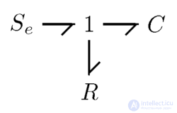
The last step — applying the causality principle to the bond graph. Applying the causality principle was explained above. The resulting bond graph is shown below.
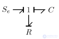
A more advanced electrical system, including a current source,
продолжение следует...
Часть 1 Bond Graph
Часть 2 Tetrahedron of State - Bond Graph
Часть 3 State equations - Bond Graph
 where
where : convergence factor










 where
where volume of the object
 : specific heat capacity at constant pressure
 where
where where
where — is the heat capacity at constant volume.
 where
where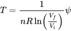 where
where : final volume
 : initial volume
 where
where : emissivity
 : Stefan-Boltzmann constant




Comments