State equations - Bond Graph

Это окончание невероятной информации про бондграф.

...

resistors, capacitors, and a transformer.

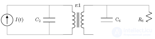
Carrying out the steps described will result in the bond graph below (before its simplification). The nodes marked with an asterisk denote the ground.

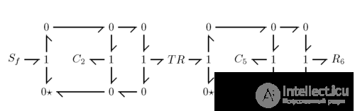
Simplifying the bond graph results in the image presented below.

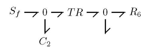
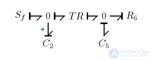
Finally, applying the causality principle results in the bond graph presented below. The bond marked with an asterisk denotes a causality conflict.

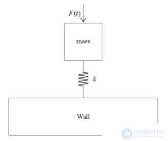
A simple linear mechanical system consisting of a mass on a spring attached to a wall. A certain force is applied to the mass. An image of the system is shown below.

For a mechanical system, the first step is to place a 1-junction at each of the various velocities; in this case there are two different velocities: the mass and the wall. Usually, for the sake of convenient notation of the 1-junctions. The result is presented below.1mass1wall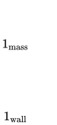

The next step is to draw the R and C bonds at their own 0-junctions between the 1-junctions where they act. In this example there is only one such bond — the C bond for the spring. It acts between the 1-junction representing the mass and the 1-junction representing the wall. The result is shown below.1mass|0−C:1k|1wall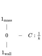

Next, the sources and I-bonds must be added at the 1-junction where they act. There is one source, a source of effort (force), and one I-bond, the mass's mass, and both of them act on the 1-junction of the mass. The result is shown below.Se:F(t)|1mass−I:m|0−C:1k|1wall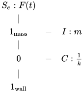

Next, the direction of energy flow must be determined. As in the electrical examples, energy must flow toward the ground, in this case toward the 1-junction on the wall. The exceptions are the R, C, or I bonds, which always point toward the element. The resulting bond graph is given below.

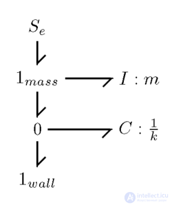
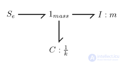
Now that the bond graph has been constructed, it can be simplified. Since the wall is grounded (has zero velocity), this node can be removed. Thus, the 0-junction on which the C bond sits can also be removed, since it would then have fewer than three bonds. The simplified bond graph is shown below.

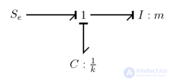
The last step — applying the causality principle; the resulting bond graph can be seen below.

A more advanced linear mechanical system is presented below.

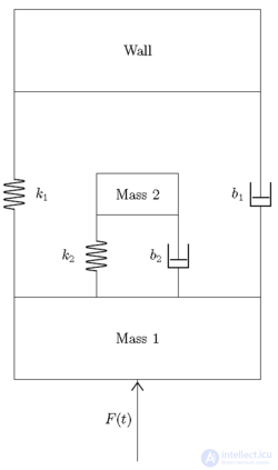
As in the example above, the first step is to create 1-junctions at each of the discrete sections with different velocities. In this example there are three discrete sections with velocity: mass 1, mass 2, and the wall. You then connect all the junctions and assign the energy flow. The junction diagram is shown below.

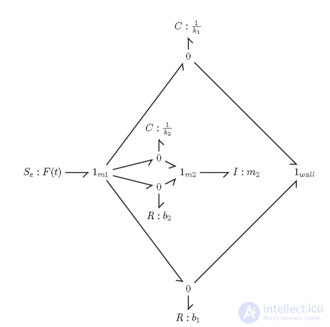
Next, you begin the process of simplifying the bond graph by removing 1-bond junctions and junctions with fewer than three bonds. The bond graph is shown below.

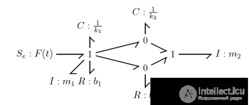
The bond graph contains a parallel power bond. Solving the parallel power bond problem was explained above. The result of the solution can be seen below.

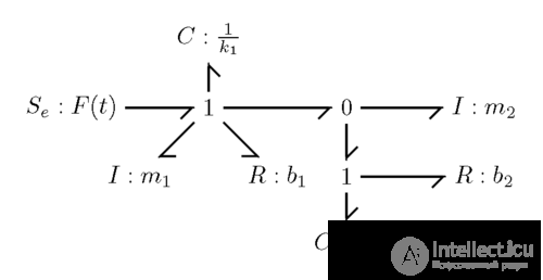
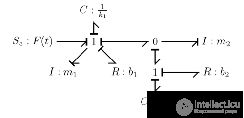
Finally, apply the causality principle; the resulting bond graph can be seen below.

Once the construction of the bond graph is complete, it can be used to generate the equations of the system in state space. The state-space representation is particularly effective because it allows complex differential systems of multi-order equations to be solved as a system of first-order equations. The general form of the state equation is as follows:x˙(t)=Ax(t)+Bu(t)wherex(t)represents the column matrix of the state variables, or the unknown parameters of the system.x˙(t)is the time derivative of the state variables.u(t)represents the column matrix of the system's input data. AndAandBrepresent matrices of constants based on the system. The state variables of the system areq(t)andp(t)the values for each C and I bond without a causality conflict. Each I bond receives the valuep(t)while each C bond receivesq(t).

For example, if you have the following bond graph

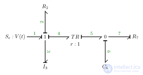
you will have the followingx˙(t),x(t), andu(t)matrices:

The matricesAandBThe state equations are solved by determining the relationship between the state variables and their corresponding elements, as described in the state tetrahedron. The first step in solving the state equations is to compile a list of all the constitutive equations for the bond graph. The table below shows the relationship between the bonds and their constitutive equations.

Element type	Bond name	Bond with causal stroke	Constitutive equation(s)
One-port elements	Source/Sink, S	Se−−−⇀|	input=e(t)
Sf|−−−⇀	input=f(t)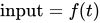
Resistance, R: Dissipated energy	−−−⇀| R	f(t)=1Re(t)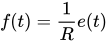
|−−−⇀ R	e(t)=Rf(t)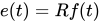
Inertia, I: Kinetic energy	♦−−−⇀| I	f(t)=1I∫e(t)dt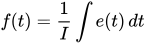
|−−−⇀ I	e(t)=If˙(t)
Compliance, C: Potential energy	−−−⇀| C	f(t)=Ce˙(t)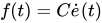
♦|−−−⇀ C	e(t)=1C∫f(t)dt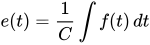
Two-port elements	Transformer, TF	−−−⇀| TF −−−⇀| r:1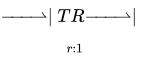	f1=1rf2 e2=1re1
| −−−⇀ TF | −−−⇀ r:1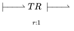	e1=re2 f2=rf1
Gyrator, GY	| −−−⇀ GY−−−⇀| g:1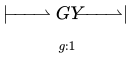	e1=gf2 e2=gf1
−−−⇀| GY|−−−⇀ g:1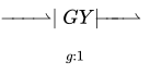	f1=1ge2 f2=1ge1
Multi-port elements	0-junction	Exactly one causal stroke at the junction	all e(t)=
1-junction	exactly one causal stroke away from the junction
all f(t)=

The symbol «♦» denotes the preferred causality.

In the example given,

The constitutive equations are as follows.

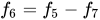
These equations can be transformed to obtain the state equations. In this example, you are trying to find the equations that relatep˙3(t)andq˙6(t)in terms ofp3(t),q6(t), ande1(t).

To begin, recall from the description of the state tetrahedron thatp˙3(t)=e3(t)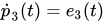Starting from equation 2, you can transform it so thate3=e1−e2−e4.e2can be substituted into equation 4, while in equation 4,f2can be replaced byf3by virtue of equation 3, which can then be replaced by equation 5.e4can likewise be replaced using equation 7, in whiche5can be replaced bye6which can then be replaced by equation 10. After these substitutions, the first state equation is obtained, which is shown below.

The second state equation can also be solved by recalling thatq 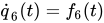The second state equation is shown below.

Both equations can be further transformed into matrix form. The result is presented below.

At this point, the equations can be treated like any other state-space representation problem.

Bond graphs have been used to model systems relevant to the biological sciences, including physiology and biology. [ 3 ] In particular, the use of bond graphs for modeling biophysical systems was proposed by Aaron Katchalsky, George Oster, and Alan Perelson in the early 1970s. [ 4 ] [ 5 ] More recently, these ideas have been used in the context of systems biology to provide an energy-based approach to modeling the biochemical reaction systems of cell biology ^{[ 6 ] [ 7 ] [ 8 ]} and to modeling the whole physiome. ^{[ 9 ]}

The bond graph method has a number of features that make it a good basis for building large computational physiome models.

• It is an energetic process, and therefore the following holds:
  • the models are physically plausible ^{[ 10 ]}
  • detailed balance (Wegscheider conditions) for reaction kinetics is satisfied automatically ^{[ 11 ]}
  • Energy flow, its use and dissipation can be considered directly.
• It is modular: bond graph components can themselves be bond graphs ^{[ 12 ] [ 13 ]}
• Energy conversion between physical domains is represented in a simplified form ^{[ 9 ]} - see below.
• Symbolic code that can be used for modelling can be generated automatically ^{[ 14 ]}

The bond graph variables for biochemical systems are as follows:

• Displacement: amount of a chemical substance, measured in moles, symbolx (mol)
• Flow: rate of change of chemical substances, symbolv (mol/s)
• Effort: chemical potential, or Gibbs energy, per mole of chemical substance, symbolμ(J/mol) ^{[ 15 ]}

Note that the product of effort and flow (μv), as always in the bond graph formulation, represents power (J/s).

As detailed below, the main features of the components used for modelling biochemical systems are as follows: components R and C are nonlinear, component I is not required, and component R is replaced by the two-port component Re. ^{[ 8 ]}

In this context, the zero (0) and one (1) bond graph junction components are no different from one another.

Component C integrates the flowvto give the amount of speciesx:

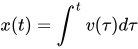
The effort, the chemical potentialμ, is given by the formula: ^{[ 8 ] [ 15 ]}

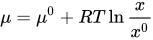
where is the chemical potential corresponding tox=x0,Ris the gas constant andT— is the absolute temperature in degrees Kelvin.

The formula forμIn simplified form this can be rewritten as follows:

where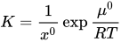

Because of the special form of this particular C component, it is sometimes given the special name Ce, by analogy with the special Re component.

The Re (reaction) component has two energy ports, corresponding to the left (forward) and right (reverse) sides of the chemical reaction. The forward sideAfand in reverse orderArAffinity is defined as the total chemical potential due respectively to the species located to the left and to the right of the reaction point. The Re component then defines the reaction flowvas: ^{[ 8 ]}

v=κ(exp⁡AfRT−exp⁡ArRT)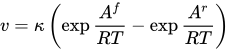

whereκ(mol/s) — is the rate constant.

Note that using the ordinary R component with a single-junction formulation is not possible, since the flow depends on both the forward and the reverse flow.Afand in reverse orderArof their similarity, not their differenceAf−Ar. ^{[ 6 ]}

Sources: ^{[ 6 ] [ 8 ]}

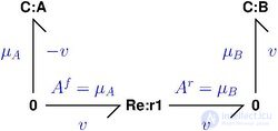
The bond graph of reactionA↽−−⇀BC:A and C:B represent species A and B, Re:r1 represents the reaction. Bonds and junctions connect the three components. The effort and flow associated with each bond are marked.

The simple reactionA↽−−⇀Bis represented by three components:

• C:A denotes species A with chemical potentialμA; the flow is−v.
• C:B denotes species B with chemical potentialμB; the flow isv.
• Re_r1 represents the reaction with flowv, forward affinityAf=μAand reverse affinityAr=μB.
• The bonds and junctions transfer chemical energy according to the specified effort and flow parameters.

Using the equations above, the flowvis given by the formula

where the indices correspond to the species. This is the simple mass action equation:

wherek+=κKA and k−=κKB.

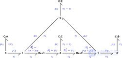
An enzyme-catalysed reaction reversibly converting species A into species B with the help of enzyme E and the enzyme complex C. The four C components represent the four species, and the two Re components represent the two reactions r1 and r2. The bond graph shows how enzyme E is recycled from the reverse side of reaction r2 to the forward side of reaction r1.

As discussed in section 1.4 of Keener and Sneyd's work ^{[ 15 ]}, the enzyme-catalysed reaction reversibly transforming speciesAinto speciesBvia enzymeEand enzyme complexCcan be represented as a pair of reactions:

The enzyme complexCis formed fromA+Eand decomposes into speciesBand releases the enzymeEThe figure shows a bond graph diagram illustrating the enzyme recycling process.

The bond graph can be used to derive the properties of these reactions, which have the generalised Michaelis-Menten form. ^{[ 6 ]}

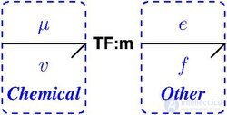
Energy conversion in the biological sciences. The TF component in the bond graph represents energy conversion either within or between energy domains. This diagram focuses on energy conversion between chemical domains with effortμ(J/mol) and flowv(mol/s) and a general domain with efforteand flowfThe transformer has modulus m.

The TF (transformer) component of the bond graph represents energy conversion either within or between energy domains. ^{[ 16 ]} (Note that the TF component is also called the TD (transduction) component ^{[ 4 ] [ 5 ]} - TF is more widely used. ^{[ 16 ]} ) This section is devoted to conversion between chemical domains with effortμ(J/mol) and flowv(mol/s) and a general domain with efforteand flowf.

A key feature of the TF component is that it transmits energy without dissipation; ^{[ 16 ]} therefore, referring to the figure:

The transformer has modulus m (with the appropriate units), such that:

From the energy formula it follows that:

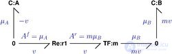
Bond graph representing the chemical reactionA↽−−⇀mB (where m is a positive integer) using the TF component.

The stoichiometry of a chemical reaction determines the amount of each chemical substance in the reaction mixture. So, for example, the reactionA↽−−⇀mBconverts one mole of substanceAinto m moles of speciesB.

The case wherem=1corresponds to the simple reaction from the first example above. Using the same approach for the general casem, the reaction flow is as follows: ^{[ 6 ] [ 8 ]}

v=κ(exp⁡μART−exp⁡mμBRT)=κ(KAxA−(KBxB)m)

This section considers the case where the general domain of definition is the electrical domain, so that the effort is expressed as (electrical) voltageV(e=V) and the flow is the current ( Consider the flowvof charged ions, where the charge of the molecule equalszϵ(coulombs), whereϵ— is the electron charge, measured in coulombs; thus, the charge associated with a mole of ions equals whereNA— is Avogadro's constant. The equivalent current is then equal to

vwhere — is Faraday's constant; therefore, the corresponding TF modulus is equal to:

(S/mol)

Again, it follows that

V

In this context, the bond graph's TF component can be used to model energy flows associated with the action potential ^{[ 17 ] ,} membrane transporters ^{[ 18 ]} , the cardiac action potential [ ^{19 ]} and the mitochondrial electron transport chain ^{[ 17 ]} .

Consider a long rigid molecule such as actin, where a subunit of lengthδ(m) is added at a ratev(mol/sec). Then the velocity of the pointed endVis given by the formula: ^{[ 20 ]}

where — is Avogadro's constant.

Thus, the modulus A(m/mol) and

where — is the corresponding force at the tip.

These formulas were used ^{[ 20 ]} to construct force/velocity curves for actin filaments. This approach represents a useful alternative to the Brownian ratchet approach ^{[ 21 ]} , since the bond graph's TF component can potentially be used with modular bond graph models of cellular systems. ^{[ 7}

Продолжение:

Часть 1 Bond Graph
Часть 2 Tetrahedron of State - Bond Graph
Часть 3 State equations - Bond Graph