
Lecture
The signal-flow graph (linear signal-flow graph, linear signal graph; English: signal-flow graph, SFG), proposed by Claude Shannon but often called the Mason graph because of his work devoted to this concept — is a specialized flow graph[eng.] in which the vertices correspond to certain variables, and the edges connect incident vertices by some functions. More formally: a directed graph, each vertex i of which corresponds to a signal (weighting function) ai, depending in some way on the signals (weighting functions) at other vertices.
Signal-flow graphs are most often used to represent the flow of signals in a physical system and its controllers, which together form a unified cyber-physical system. They are also used in various electronic networks and amplifiers, in digital filters, state-variable filters, and in certain types of analog filters. In the literature, signal-flow graphs are usually associated with a system of linear equations.
Wai-Kai Chen wrote: «The concept of the signal-flow graph was developed by Shannon . while working with analog computers. The greatest contribution to the development of the signal-flow graph belongs to Mason . He showed how to use the signal-flow graph to solve certain complex electronic problems in a relatively simple way. The term signal-flow graph was used because of its original application to electronics and its resemblance to electronic signals and the block diagrams of the systems being studied».
Lorens wrote: «Before Mason's work, Shannon identified a number of properties of what is now known as flow graphs. Unfortunately, the document was initially very limited in its distribution, and very few people had access to the materials».
«The rules for computing the determinant of Mason's graph were first given and proved by Shannon using mathematical induction. His work remained practically unknown even after Mason published his classic paper in 1953. Three years later Mason independently rediscovered the rules and proved them by considering the value of the determinant and how it changes when variables are added to the graph. [...]»
Robichaud et al. define the scope of application of the signal-flow graph as follows:
«The scope of application of the developed methods comprises all physical systems analogous to these networks [built from ideal transformers, active elements and gyrators]. Trent showed that all physical systems satisfying the following conditions fall into this category.
- A finite lumped system consists of a number of simple parts, each of which has known dynamic properties that can be determined by equations using two types of scalar variables and system parameters. Variables of the first type represent quantities that can be measured, at least in principle, by connecting a measuring instrument to two junction points of the element. Variables of the second type characterize quantities that can be measured by connecting a meter in series with the element. Relative velocities and positions, pressure drops and voltages are typical quantities of the first type, whereas electric currents, forces, and heat-flow rates are quantities of the second type. [...]
- Variables of the first type must obey a law analogous to Kirchhoff's voltage rule, whereas variables of the second type must obey a law analogous to Kirchhoff's node (current) rule.
- The physical dimensions of the corresponding computed results of the variables of both types must be consistent. For systems in which these conditions hold, a linear graph can be constructed that is isomorphic to the dynamic properties of the system described by the chosen variables. These methods [...] can be applied directly to these linear graphs, just as to electrical networks, to obtain the signal-flow graph of the system.»
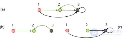
(a) flow graph, (b) edges entering node 2, (c) edges entering node 3
In the graph shown in the figure, the functional dependence of a node is indicated by an arrow entering it, while the node giving rise to this dependence is the origin of that arrow; in its most general form, the signal-flow graph shows by incoming arrows only those nodes that affect the processing at the receiving node, and at each i-th node the incoming variables are processed according to the function associated with that node, for example Fi. Thus, (a) represents the set of explicit relations:
x1=independent variable 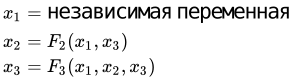
Node x1 is an isolated node, since no arrow enters it; the equations for x2 and x3 correspond to the graphs shown in parts (b) and (c) of the figure.
These relations define, for each node, a function that processes the input signals received by the node. Every node that is not a source combines the input signals in some way and transmits the resulting signal along each outgoing branch. «A flow graph, as originally defined by Mason, implies a set of functional relations, linear or not» .
However, Mason's graphs are usually more strict, implying that each node only sums the arrows entering it, and that each edge is a function only of the node from which it originates. Under these conditions the system is written as follows:
x1=independent variable 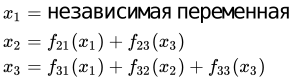
Now the functions  can be assigned to
  an edge of the signal-flow graph connecting a pair of nodes
  ,
,  , instead of defining general functions for each node. A node's contribution to itself, for example
  for
for  , is called a loop. Often these functions are simply multiplicative coefficients (often called transmittances or gains), for example,
 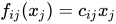 , where c
 - can be not only a scalar, but also a function of some parameter, such as the Laplace transform variable s
 . Signal-flow graphs are very often used with Laplace-transformed signals, since they represent systems of linear differential equations. In this case the transmittance c(s) is often called the transfer function.
There are several ways to choose variables in a complex system, and for each of them a system of equations can be written that can be represented as a graph. Writing the equations is greatly facilitated if there is a method that allows the graph to be constructed directly from the schematic diagram of the system under study. The structure of the graphs obtained in this way is obviously related to the topology of the schematic diagram, and even implicit consideration of the equations becomes unnecessary. In some cases it is sufficient simply to represent the flow graph on the schematic diagram and to arrive at the solution of the problem even without a drawing.
The signal-flow graph contains the same amount of information as the equations from which it is derived; but there is no one-to-one correspondence between the graph and the system of equations. The same system will yield different graphs depending on the order in which the equations are used to find the variable written on the left-hand side. For example, if each equation relates all n dependent variables, then there exist n!
 possible graphs.
The methods of the linear signal-flow graph apply only to linear time-invariant systems. When modeling the system of interest, the first step is usually to determine the equations representing the operation of the system, regardless of their nature. The graph itself is then constructed on the basis of this system of equations.
A linear signal-flow graph consists of nodes and weighted directed branches. The nodes are the variables of the equations, and the branch weights are the coefficients. Signals can flow along a branch only in the direction indicated by the arrow. The graph can represent only the operations of multiplication by a coefficient and addition, which are sufficient to represent the coupling equations. When a signal crosses a branch in the indicated direction, the signal is multiplied by the branch weight. When two or more branches are directed into the same node, their outputs are summed.
For systems described by linear algebraic or differential equations, the signal-flow graph is mathematically equivalent to the system of equations describing the system. In this case, the equations defining the graph can be found for each node by summing the branches entering that node. The branches themselves carry the contributions of other nodes, expressed as the value of the source node multiplied by the weight of the connecting branch, which is usually a real number or a function of some parameter (for example, the Laplace transform variable s).
Choma, an IEEE member, wrote the following regarding linear active networks:
«By a signal-flow representation (or «graph», as it is usually called) we mean a diagram which, by displaying the algebraic relations between the corresponding variables and branches of the network, unambiguously represents how an applied input signal «flows» from the input ports to the output ports [...]» .
The usefulness of signal-flow graph analysis was also described by computer scientist Chen:
«The analysis of a linear system ultimately reduces to solving a system of linear algebraic equations. As an alternative to the usual algebraic methods of solving the system, a solution can be obtained by considering the properties of certain directed graphs associated with the system. [...] The unknowns of the equations correspond to the nodes of the graph, while the linear relations between them appear as directed edges connecting the nodes. [...] The associated directed graphs can in many cases be composed directly by inspection of the physical system, without first having to formulate the corresponding equations»[10].

Comments