Types of Inputs. Step Response, Impulse Response, Transfer Function
- Unit step function — a special mathematical function whose value equals zero for negative arguments and one for positive arguments. It is the natural, simplest input applied to a controlled object. In mathematics it is expressed as the Heaviside unit function.
- Unit impulse function — the derivative of the unit step function. It characterizes a pulse of infinitely large amplitude acting over an infinitely small time interval. Geometrically, the area bounded by this function equals 1. It is used in a number of cases where determining dynamic characteristics by the simplest method is impossible because the output value would exceed the specified value.
- Step response — the response of a system to a unit step signal.
- Impulse response — the response of a system to a unit impulse.
- Transfer function — the ratio of the Laplace transform of the output signal to the Laplace transform of the input signal under zero initial conditions and zero external disturbances.
Transfer Function of a Connection of Elements
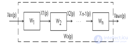
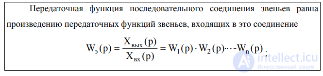
Series Connection
Weq(p) = W1(p)W2(p)…Wn(p) =  (p)
(p)
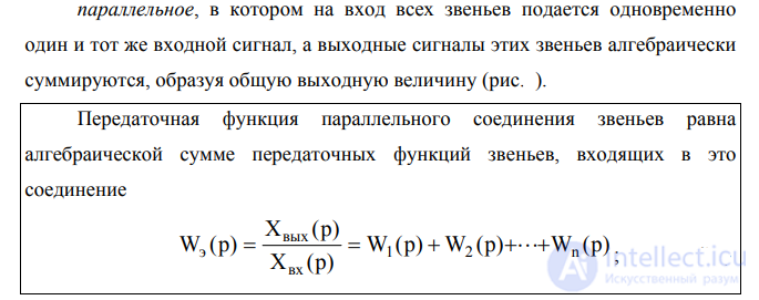
Parallel Connection
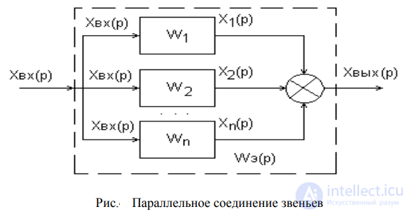
Weq(p) = W1(p) + W2(p) + … + Wn(p) =  (p)
(p)
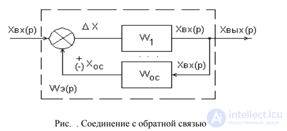
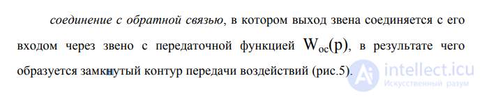
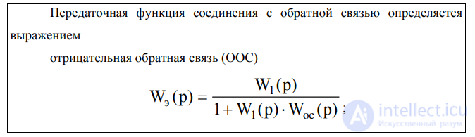
Transfer Function of a Feedback Connection

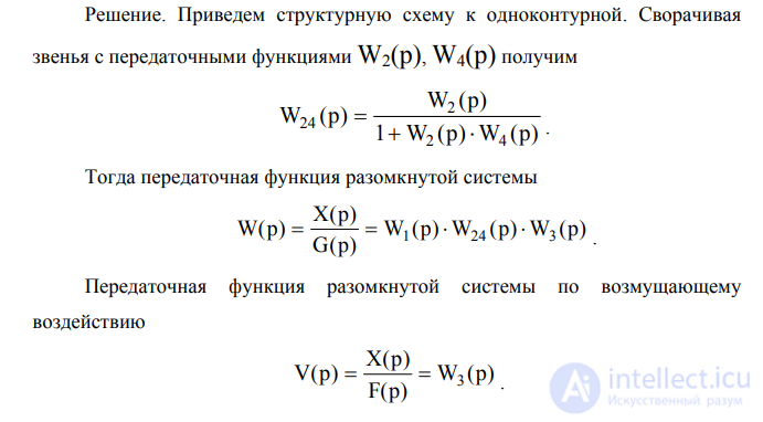
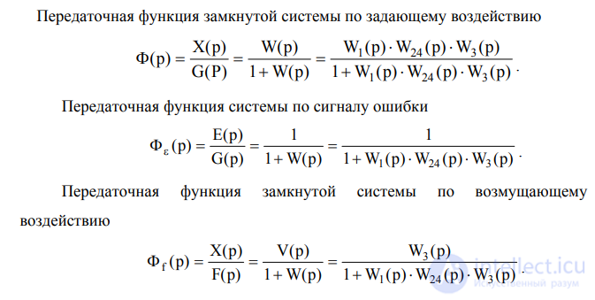
Example: find the transfer function of a system from its block diagram
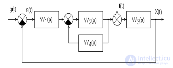
Fig. Block diagram of the ACS
Transfer Function of a Closed-Loop System
- WFB(p) — the equation describing the feedback loop
- W(p) — the equation describing the element
- G(p) — the equation describing the input action
- UFB(p) — the equation describing the output signal of the feedback element
- ΔU(p) — the equation describing the sum (difference) of G(p) and UFB(p)
- Y(p) — the equation describing the output signal of the system
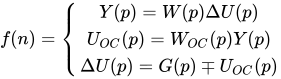
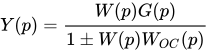
Solving this system of equations, we obtain the following results:



Obtaining the Transfer Function in State Space
A system in state space is given in the form:
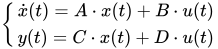
The system has m inputs u(t), l outputs y(t), n states x(t), n>= max(m, l), A,B,C,D — numerical matrices of the corresponding dimensions nxn, nxm, lxn, lxm..
Let I — the identity matrix of dimension nxn, then:
pI X(p) — A X(p) = B U(p)
(pI — A)X(p) = BU(p)
x(0) = 0
X(p)=Wxu(p)U(p); Wxu(p) = (pI — A)^{-1)B
Y(p)=Wyu(p)U(p); Wyu(p)=C (pI — A)^{-1) B + D
Linearization of Systems and Elements
Let an ACS be controlled and described by a nonlinear equation

Moreover, the nonlinearity is insignificant, i.e. this function can be expanded in a Taylor series in the neighborhood of a stationary point, for example, at zero external disturbance f = 0.
The equation of this element in steady state is as follows:
 , initial points, no derivatives.
Then, expanding the nonlinear function in a Taylor series, we obtain:
 — the remainder term

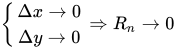

We have moved from a nonlinear notation to a linear one. Let us proceed to the operator equation:


See also
- Block diagram
- Transformation of block diagrams
- [[b6726]]
- [[b6512]]
- [[b6931]]


Comments