
Lecture
Control laws are relationships, established by theoretical or empirical means and logically substantiated, between the goals of management activity and the methods of achieving them.
A control law is an algorithm or functional relationship according to which the controller forms the control action u(t). This relationship can be represented in the form
u(t) = F(x, g, f), (8.1) (explanation below)
A regularity – a necessary, essential, constantly recurring interrelation of phenomena of the real world that determines the stages and forms of the process by which phenomena of nature, society and spiritual culture emerge and develop.
According to established practice, control laws are customarily divided into three main groups.
The first group comprises general (objective) control laws. Objective control laws are usually understood to be laws inherent to management as a whole, expressing relationships that form independently of the will of individual subjects.
The second group includes particular, or subjective, control laws, the application of which can significantly increase the efficiency of the control system's functioning as a whole, as well as of its individual elements and units. Subjective control laws include the law of change of management functions, the law of reduction in the number of management levels, and the law of the extent of control.
Finally, the third group should reasonably include laws not directly related to management but capable of exerting a significant influence on the results of an organization's activity. The laws of the third group include economic, legal, social and other laws. Such laws can be designated by the term "special".
Suppose that the block diagram of such an ACS consists of a certain number of elements (blocks). Grouping the blocks by functional principle (what the blocks do), the block diagram of the ACS can be reduced to the following typical form:
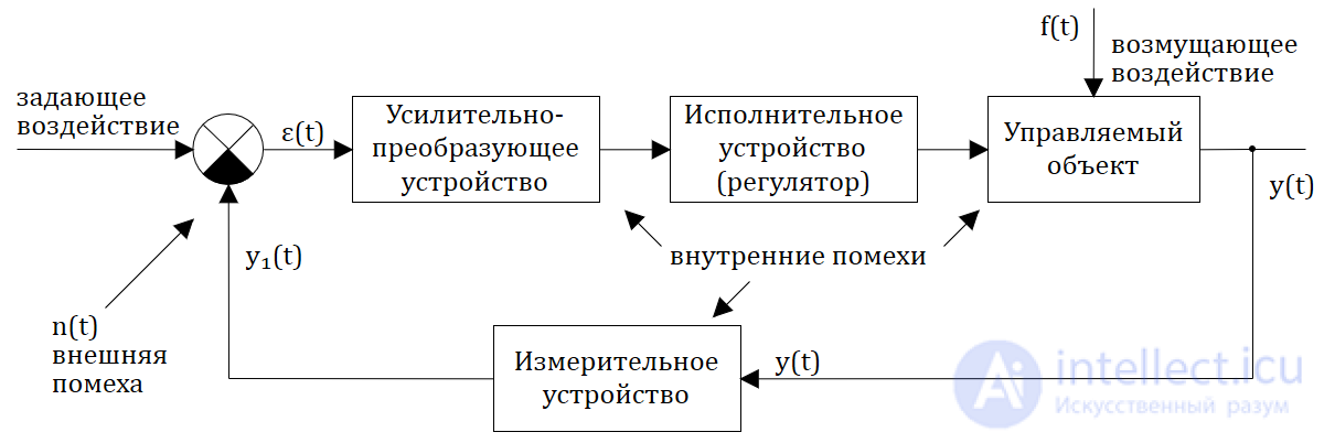
Fig. 1.2.3 — Block diagram of an automatic control system
The symbol ε(t) or the variable ε(t) denotes the discrepancy (error) at the output of the comparing device, which can “operate” in the mode of both simple comparative arithmetic operations (most often subtraction, less often addition) and more complex comparative operations (procedures).
Since y1(t) = y(t)*k1, where k1 — the gain factor, then ==>
ε(t) = x(t) — y1(t) = x(t) — k1*y(t)
The task of the control system is (if it is stable) to “work” toward eliminating the discrepancy (error) ε(t), i.e. ==> ε(t) → 0.
It should be noted that the control system is affected both by external actions (control action, disturbance, noise) and by internal noise. A disturbance differs from an action in the stochastic (random) nature of its existence, whereas an action is almost always deterministic.
To denote the control (reference) action we will use either x(t), or u(t).
If we return to the last figure (the block diagram of the ACS in Fig. 1.2.3), it is necessary to “decode” the role played by the amplifying-converting device (what functions it performs).
If the amplifying-converting device (ACD) performs only amplification (or attenuation) of the discrepancy signal ε(t), namely: 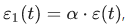 , where α– is the proportionality coefficient (in the particular case α = Const), then such a control mode of the closed-loop ACS is called the mode of proportional control (P-control).
If the ACD forms an output signal ε1(t) proportional to the error ε(t) and to the integral of ε(t), i.e.  , then such a control mode is called proportional-integrating (PI-control). ==>
  , where b – is the proportionality coefficient (in the particular case b = Const).
PI-control is usually used to increase the accuracy of control (regulation).
If the ACD forms an output signal ε1(t) proportional to the error ε(t) and to its derivative, then such a mode is called proportional-differentiating (PD-control): ==> 
The use of PD-control usually increases the speed of response of the ACS
If the ACD forms an output signal ε1(t) proportional to the error ε(t), its derivative, and the integral of the error ==> , then such a control mode is called the proportional-integral-derivative control mode (PID-control).
PID-control often makes it possible to provide “good” control accuracy together with “good” speed of response.
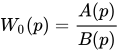
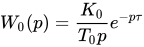
Statistical models are characterized by a set of statistical parameters and distribution functions. Methods of mathematical statistics are used to study them.
Adaptive models use deterministic-stochastic methods to describe the controlled object.
Hypotheses and analogues that reflect the real, objectively existing world must possess clarity or be reducible to logical schemes convenient for research: such logical schemes, which simplify reasoning and logical constructions or allow experiments to be carried out that clarify the nature of phenomena, are called models. In other words, a model (Lat. modulus – measure) – is an object – a substitute object – for the original object, providing for the study of certain properties of the original.
By mathematical modeling we mean the process of establishing a correspondence between a given real object and a certain mathematical object, called a mathematical model, and the study of this model, which makes it possible to obtain the characteristics of the real object under consideration. The form of the mathematical model depends both on the nature of the real object and on the objectives of studying the object and the required reliability and accuracy of the solution to this problem.
Differential equations are used for the mathematical modeling of linear continuous ACS.
In continuous systems, both the input actions and the output processes are continuous functions. The relationship between them is expressed by means of differential equations of the following form:
|
|
(1) |
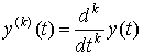
wherex(t) andy(t) – are the reference action and the output process, and the variables 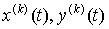 - are their derivatives. If the functionsF1 andF2 – are nonlinear with respect to the variables, then the systems will be nonlinear.
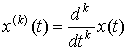
In linear systemsF1 andF2 – are linear functions. If they explicitly depend on timet, then the systems will be non-stationary. In the case of stationary systems, there is no explicit dependence of the functions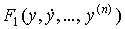 and
and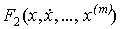 on time. The order of the highest derivativen of the output variable in the left-hand side of the equation is called the order of the equation or the order of the system.
If a stationary system admits linearization of its equations, then it is described by a linear differential equation of the following form:
|
|
(2) |
where c andb – are constant coefficients depending on the system's parameters. All the variables enter this equation linearly, which ensures that the principle of superposition is applicable to the system.
Thus, if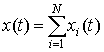 , then the output process
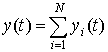 , where equation (2) corresponds to each pair xi(t) and yi(t).
An example of equation (2) is the linearized equation:
 .
.
If we denote

then we obtain a particular case of equation (2).
The analysis of a linear stationary system reduces to finding the functiony(t) for a given actionx(t). In other words, the analysis of the ACS requires finding the solution of equation (2). It is known from the corresponding sections of higher mathematics that the solution of equation (2) consists of two terms:
 ,
,
whereytr(t) is the transient component of the solution, or the transient process of the system, which is found from the solution of the homogeneous equation
|
|
(3) |
under zero initial conditions for the process itself and its first (n-1) derivatives.
Let us explain the meaning of the transient process in an ACS using the example of a PLL tracking system. The linearized equation of this system is equal to
|
|
(4) |
where x(t) = jx(t) – is the phase of the input action of the signal generator SG, and y(t) = = jy(t) – is the phase of the output signal of the tunable generator TG.
Let the reference action x(t) = 0, and at the moment the system is switched on, when t = 0 the output phase y(t)  0.
0.
Owing to the presence of an initial discrepancy

the system begins to operate, striving to ensure the value of the phase of the output
process y(t) = x(t) = 0. This will be the transient processy tr(t).
Since, by condition, the actionx(t) = 0, equation (4) for the transient process takes the form
 ,
,
which is a homogeneous equation for (4).
Its solution is easily found and has the form
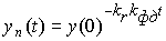 .
.
The exponential character of the transient process is shown in Fig. 11.
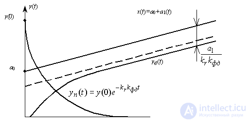
Fig. 11. Transient and forced processes in a PLL system
Now let us consider the forced processyf(t). It is determined only by the reference actionx(t) under zero initial conditions in the system. To findyf(t) it is necessary to determine a particular solution of the inhomogeneous equation
|
|
(5) |
under zero initial conditions and a given functionx(t).
For the PLL system under consideration, the equation of the forced process takes the form
 .
.
As an example, let us assume

Using the expression for the general solution of a first-order differential equation, we can write that
 .
.
From this it is easy to obtain the forced process of the PLL, assuming
y(t) = 0; x(t) = a0 + a1t:
 .
.
The character of this relationship is shown in Fig. 11. As time passes, at t the output process will tend to the function
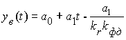 ,
,
that is, the phase of the output signal will be less than the phase of the input by the amounta1/krkpd and the tracking system will operate with a certain error.
It is important to emphasize that, owing to the zero initial conditions, the forced processyf(t) starts from zero.
On the basis of the superposition principle, the resulting process in the system
y(t) = ytr(t) + yf(t).
Thus, the study of linear stationary automatic control systems reduces to a separate study of the characteristics of the transient and forced processes, the methods for determining which, as a rule, turn out to be different.
A control law is an algorithm or functional relationship according to which the controller forms the control action u(t). This relationship can be represented in the form
u(t) = F(x, g, f), (8.1)
where F is a certain operator of the deviation x, the reference action g and the disturbance action f, as well as of their derivatives and integrals with respect to time.
Usually expression (8.1) can be written as follows:
u(t) = F1(x) + F2(g) + F3(f). (8.2)
Here the first term corresponds to control by deviation, and the second and third to control by external action.
Depending on the form of the operator F, control laws are divided into standard and special ones.
Standard control laws are universal laws by means of which it is possible to solve problems of automating a variety of technological processes and objects.
Special control laws are laws formulated to solve specific problems.
If only linear mathematical operations are used to form the control action u(t), then such a control law is called linear; otherwise it is called nonlinear.
A linear standard control law has the following form:
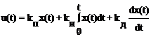 , (8.3)
where the first term is the proportional, the second the integral, and the third the derivative component of the law, and the coefficients kP, kI and kD determine the contribution of each component to the control action being formed.
The integral component of the control law is introduced to increase accuracy, and the derivative component to increase the speed of response of the system.
A controller that forms the control action in accordance with (8.3) has the transfer function
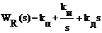 . (8.4)
The block diagram of a linear standard controller is shown in Fig. 8.1.
Tuning such a controller consists in setting the values of the coefficients kP, kI, kD in such a way as to satisfy the requirements for the quality of control in accordance with the chosen quality criteria.
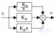
Fig. 8.1. Structure of a linear standard controller
In practice, standard or industrial controllers have become widespread; these are universal automatic devices that are easily adapted for automating a variety of technological processes and objects. In this case the controlled object is, as a rule, a static-type element, i.e. Wpl(0)=kpl, where kpl is the transfer coefficient of the controlled object. Standard controllers implement standard control laws, which are particular cases of the linear standard control law, and are classified as follows.
P-controllers. They implement the P-law, or proportional control law
u(t) = kP x(t).
The transfer function of a P-controller
WR(s) = kP.
Proportional control makes it possible to reduce the steady-state error in the object by a factor of (1+k), where k = kP´kpl is the transfer coefficient of the open-loop system. Control in this case turns out to be static, since for any finite value of the open-loop transfer coefficient the steady-state error will be nonzero.
I-controllers. They implement the I-law, or integral control law
u(t) = 
 .
.
The transfer function of an I-controller
 .
.
With integral control, the system obtained is astatic with respect to the reference action. Increasing the degree of astatism leads to an increase in the steady-state accuracy of the system, but at the same time reduces its speed of response and also worsens its stability. The decrease in speed of response is explained by the fact that at the first moment in time, when an error appears, the control action equals zero and only then does it begin to grow. In a proportional control system, the growth of the control action in the first moments of time occurs more intensively, since the presence of an error immediately produces a control action, whereas in an integral control system some time must pass.
PI-controllers. They implement the PI-law, or proportional-integral control law
u(t) = kP x(t) +.
The transfer function of a PI-controller
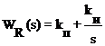
 ,
,
where TI = kP/ kI.
Proportional-integral (isodromic) control combines the high accuracy of integral control (astatism) with the high speed of response of proportional control. In the first moments of time, when an error appears, a system with a PI-controller operates as a proportional control system, and later begins to operate as an integral control system.
PD-controllers. They implement the PD-law, or proportional-derivative control law
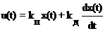 .
.
The transfer function of a PD-controller
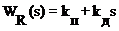 = kP(TDs + 1),
where TD = kD/ kP.
Proportional-derivative control is used to increase the speed of response of the system.
Control based on the derivative has no independent significance, since in the steady state the derivative of the error is equal to zero and control ceases. However, it plays a major role in transient processes, because it makes it possible to take into account the tendency of the error to increase or decrease. As a result, the response speed of the system increases, the speed of response is improved, and the dynamic error is reduced.
PID-controllers. They implement the PID-law, or proportional-integral-derivative control law, corresponding to the linear standard law of the form (8.3).
A PID-controller, which is an astatic isodromic controller with anticipation, provides increased accuracy and increased speed of response of the system.
 ;
; ;
;  ,
,




Comments