
Lecture
Theory of Automatic Control (TAC) — a scientific discipline that studies the processes of automatic control of objects of various physical nature. In doing so, mathematical means are used to reveal the properties of automatic control systems and to develop recommendations for their design.
It is an integral part of technical cybernetics and is intended for developing the general principles of automatic control, as well as methods of analysis (studying the functioning) and synthesis (selecting parameters) of automatic control systems (ACS) for technical objects.
For this theory, only the nature of the transformations of signals by the controlled objects is of significance.
The first information about automata appeared at the beginning of our era in the works of Hero of Alexandria, «Pneumatics» and «Mechanics», which describe automata created by Hero himself and his teacher Ctesibius: a pneumatic automaton for opening temple doors, a water organ, an automaton for selling holy water, and others. Hero's ideas were far ahead of their time and found no application in his era.
In the Middle Ages, imitative «android» mechanics developed significantly, when mechanic-designers created a number of automata that mimicked individual human actions, and, to enhance the impression, inventors gave the automata an external resemblance to humans and called them «androids», that is, human-like. Nowadays such devices are called robots, as distinct from the widely used automatic control devices found in all spheres of human activity, which are called automata.
In the 13th century, the German scholastic philosopher and alchemist Albertus Magnus von Bollstadt built a robot for opening and closing doors.
Very interesting androids were created in the 17th—18th centuries. In the 18th century, the Swiss watchmakers Pierre Jaquet-Droz and his son Henri created a mechanical scribe, a mechanical artist, and others. A wonderful theater of automata was created in the 18th century by the self-taught Russian mechanic Kulibin. His theater, kept in the Hermitage, is housed inside an «egg-shaped clock figure».
In embryonic form, many principles of the theory of automatic control are contained in the General Theory of (Linear) Governors, which was developed mainly between 1868—1876 in the works of Maxwell and Vyshnegradsky. Vyshnegradsky's foundational works are: «On the General Theory of Governors», «On Indirect-Acting Governors». These works contain the origins of modern engineering methods for studying stability and control quality.
A decisive influence on the development of domestic research methodology in the theory of automatic control was exerted by the works of the outstanding Soviet mathematician Andrey Markov (Jr.), founder of the Soviet constructivist school of mathematics, author of works on the theory of algorithms and mathematical logic. These studies found application in the scientific and practical work of academician Lebedev on military topics — torpedo control and gun-laying automata and the stability of large power systems.
By the beginning of the 20th century and in its first decade, the theory of automatic control was formed as a general scientific discipline with a number of applied branches.
Automation — a branch of science and technology covering the theory and practice of automatic control, as well as the principles of building automatic systems and the technical means that constitute them.
Controlled object (CO) — a device, physical process, or set of processes that need to be controlled in order to obtain the required result. Interaction with the CO takes place by applying a control action to its conditional input (which corrects the processes occurring in the CO), while at the output a changed parameter is obtained (which is a consequential process).
Control — an action (signal) applied to the input of the controlled object and ensuring such a course of processes in the controlled object as will achieve the specified control goal at its output.
Goal — the desired course of processes in the controlled object and the achievement of the required change of the parameter at its output.
Objects:
An automatic control system (ACS) includes the controlled object and the control device.
Control device — a set of devices by means of which control of the inputs of the controlled object is carried out.
Regulation — a special case of control whose goal consists in maintaining one or more outputs of the controlled object at a specified level.
Controller — converts the control error ε(t) into a control action supplied to the controlled object.
Reference input g(t) — defines the required control law of the output quantity.
Control error ε(t) = g(t) — y(t), the difference between the required value of the controlled quantity and its current value. If ε(t) differs from zero, then this signal is fed to the input of the controller, which forms such a control action that, eventually, over time, ε(t) = 0.
Disturbance f(t) — a process at the input of the controlled object that acts as interference to control.
Automatic control systems:
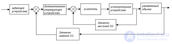
Typical ACS diagram
Functional diagram of an element — a diagram of an automatic regulation and control system, drawn up according to the function performed by the given element.
Output signals — parameters characterizing the state of the controlled object and significant for the control process.
System outputs — points of the system at which the output signals can be observed in the form of certain physical quantities.
System inputs — points of the system at which external actions are applied.
Input signals:
Systems:
Feedback — a connection in which the actual value of the output variable, as well as the specified value of the controlled variable, is fed to the input of the controller.
Control by the principle of deviation of the controlled variable — feedback forms a closed loop. An action proportional to the sum (difference) between the output variable and the specified value is applied to the controlled object, so that this sum (difference) decreases.
Control by the principle of disturbance compensation — a signal proportional to the disturbance is fed to the input of the controller. There is no dependence between the control action and the result of this action on the object.
Control by the principle of combined regulation — disturbance-based and deviation-based regulation are used simultaneously, which provides the highest control accuracy.
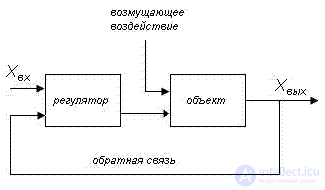
The principle of controlled-variable deviation in TAC
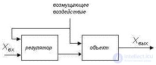
The principle of disturbance compensation in TAC
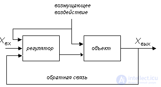
The principle of combined regulation in TAC
By the nature of control:
By the nature of action:
By the degree of use of information about the state of the controlled object:
By the degree of use of information about the parameters and structure of the controlled object:
By the degree of coordinate transformation in the ACS:
By the type of mathematical model of coordinate transformation:
By the type of control actions:
By the degree of human involvement:
By the law of change of the output variable:
By the number of controlled and regulated variables:
By the degree of self-tuning, adaptation, optimization and intelligence:
By the action of the sensing (measuring) element on the actuating element:
IACS — these are systems that allow learning, adaptation or tuning to be carried out by storing and analyzing information about the behavior of the object, its control device, and external actions. A distinctive feature of these systems is the presence of a knowledge base, an inference engine, an explanation subsystem, and others.
Knowledge base — formalized rules in the form of logical formulas, tables, etc. The IACS is used for controlling poorly formalized or complex technical objects.
A system is classified as an IACS if it satisfies the following criteria:
If the IACS satisfies all 5 criteria, then it is intelligent in the «broad» sense, otherwise in the «narrow» sense.
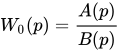
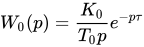
Statistical models are characterized by a set of statistical parameters and distribution functions. Methods of mathematical statistics are used to study them.
Adaptive models use deterministic-stochastic methods to describe the controlled object.
Weq(p) = W1(p)W2(p)…Wn(p) =  (p)
(p)
Weq(p) = W1(p) + W2(p) + … + Wn(p) =  (p)
(p)
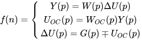
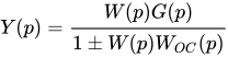
Solving this system of equations, we obtain the following results:



The state-space system is given in the form:
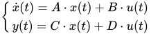
The system has m inputs u(t), l outputs y(t), n states x(t), n>= max(m, l), A,B,C,D — numerical matrices of the corresponding dimension nxn, nxm, lxn, lxm..
Let I — the identity matrix of dimension nxn, then:
pI X(p) — A X(p) = B U(p)
(pI — A)X(p) = BU(p)
x(0) = 0
X(p)=Wxu(p)U(p); Wxu(p) = (pI — A)^{-1)B
Y(p)=Wyu(p)U(p); Wyu(p)=C (pI — A)^{-1) B + D
Let the ACS be regulated and described by a nonlinear equation

Moreover, the nonlinearity is insignificant, that is, this function can be expanded in a Taylor series in the vicinity of the stationary point, for example, for an external disturbance f = 0.
The equation of this element in steady state is as follows:
 , initial point, derivatives are absent.
Then, expanding the nonlinear function in a Taylor series, we obtain:
 — the remainder term

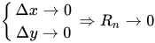

We have gone from the nonlinear notation to the linear one. Let us move on to the operator equation:


An ACS is controllable (completely controllable) if it can be transferred from any initial state x0(t) to any other arbitrary state x1(t) at an arbitrary moment of time by applying a piecewise-continuous input U(t)∈[t0;t1].
An ACS is observable (completely observable) if all state variables x(t) can be determined from the output (measured) signal y(t).
Stability — the property of an ACS to return to a specified or close-to-it steady-state mode after some disturbance. A stable ACS is a system in which the transient processes are decaying.
 — the operator form of the linearized equation.
y(t) = yss(t)+ytr = yforced(t)+yfree
yss(yforced) — the particular solution of the linearized equation.
ytr(yfree) — the general solution of the linearized equation as a homogeneous differential equation, that is 
An ACS is stable if the transient processes yn(t), caused by any disturbances, decay with time, that is  as
as 
Solving the differential equation in the general case, we obtain complex roots pi, pi+1 = ±αi ± jβi
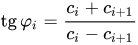
Each pair of complex-conjugate roots corresponds to the following component of the transient-process equation:
 , where
 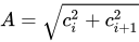 ,
, 
From the results obtained, it can be seen that:
 , which leads to diverging oscillations;
 , which leads to undamped sinusoidal oscillations of the system (the system is at the stability boundary) (Lyapunov's theorem 3).
To determine the stability of the system, tables of the following form are constructed:
| Coefficients | Rows | column 1 | column 2 | column 3 |
|---|---|---|---|---|
| 1 |  |
 |
 |
|
| 2 |  |
 |
 |
|
 |
3 |  |
 |
 |
 |
4 |  |
 |
 |
For the system to be stable, it is necessary that all elements of the first column have positive values; if the first column contains negative elements, the system is unstable; if at least one element is equal to zero while the rest are positive, then the system is at the stability boundary.

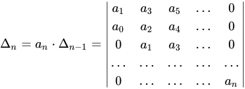 — the Hurwitz determinant
Theorem: for the stability of a closed-loop ACS it is necessary and sufficient that the Hurwitz determinant and all its minors be positive for 
Let us substitute  , where ω — is the angular frequency of oscillations corresponding to the purely imaginary root of this characteristic polynomial.



Criterion: for the stability of a linear system of the n-th order it is necessary and sufficient that the Mikhailov curve, plotted in the coordinates  , pass successively through n quadrants.


Let us consider the relationship between the Mikhailov curve and the signs of its roots (α>0 and β>0)
1) The root of the characteristic equation is a negative real number 
The factor corresponding to this root 
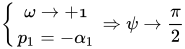
2) The root of the characteristic equation is a positive real number 
The factor corresponding to this root 
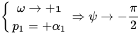
3) The root of the characteristic equation is a complex pair of numbers with a negative real part 
The factor corresponding to this root 
 , where
4) The root of the characteristic equation is a complex pair of numbers with a positive real part 
The factor corresponding to this root 
 , where
The Nyquist criterion is a graphical-analytical criterion. Its characteristic feature is that the conclusion about the stability or instability of a closed-loop system is drawn based on the shape of the amplitude-phase or logarithmic frequency characteristics of the open-loop system.
Let the open-loop system be represented as a polynomial 
then let us make the substitution and obtain: 
For a more convenient construction of the hodograph when n>2, let us reduce equation (*) to the «standard» form: 
With this representation, the magnitude A(ω) = | W(jω)| is equal to the ratio of the magnitudes of the numerator and denominator, and the argument (phase) ψ(ω) — to the difference of their arguments. In turn, the magnitude of the product of complex numbers equals the product of the magnitudes, and the argument — the sum of the arguments.
Magnitudes and arguments corresponding to the factors of the transfer function:
| Factor |  |
 |
|---|---|---|
| k | k | 0 |
| p | ω |  |
 |
 |
 |
 |
 |
 |
 |
|
 |
 |
|
 |
 |
 |
|
 |
 |
|
After that, let us plot the hodograph for the auxiliary function  , for which we will vary
For  , and for
  (since n<m and
  )
)
To determine the resulting rotation angle, let us find the difference between the arguments of the numerator  and the denominator
The numerator polynomial of the auxiliary function has the same degree as the polynomial of its denominator, from which it follows that  , and therefore the resulting rotation angle of the auxiliary function equals 0. This means that for the stability of the closed-loop system, the hodograph of the auxiliary-function vector must not encircle the origin, and the hodograph of the function
  , correspondingly, the point with coordinates
Under operating conditions, the system parameters may, for one reason or another, vary within certain limits (aging, temperature fluctuations, etc.). These parameter fluctuations can lead to a loss of stability if the system operates close to the stability boundary. Therefore, engineers strive to design the system so that it operates far from the stability boundary. The degree of this distance is called the stability margin.
The need for a stability margin is determined by the following conditions:
The frequency-domain Nyquist criterion is mainly applicable when it is difficult to obtain the phase characteristics experimentally. However, calculating the amplitude-phase characteristic (APC), especially the frequency one, is more difficult than constructing Mikhailov curves. Moreover, the position of the amplitude-phase frequency response does not give a direct answer to the question of whether the system is stable, that is, an additional study of the stability of the open-loop system is required.
The Mikhailov criterion is applicable to systems of any order, unlike the Routh criterion. By applying the frequency-domain Nyquist criterion and the Mikhailov criterion, the characteristic curves can be constructed gradually, taking into account the influence of each element, which gives the criteria clarity and solves the problem of selecting system parameters from the stability condition.
A control systems engineer's career begins with a bachelor's degree and can continue through further college study. A controls-engineering degree combines well with a degree in electrical or mechanical engineering. Controls engineers typically find work in technical management, where they often lead interdisciplinary projects. There are many employment opportunities at aerospace companies, manufacturing companies, automotive companies, energy companies, and government agencies. Some places that hire controls engineers include companies such as Rockwell Automation, NASA, Ford, and Goodrich. Controls engineers can earn $66 thousand a year at Lockheed Martin Corp. They can also earn up to $96 thousand a year at General Motors Corporation.
According to a survey by Control Engineering , most of the people who responded were controls engineers in various forms throughout their careers. There are not that many professions that can be classified under the category of «control engineer»; most of them are specific careers that bear little resemblance to the all-encompassing career of a control engineer. Most control systems engineers who took part in the 2019 survey are systems or product designers, or even instrumentation or controls engineers. Most of the work is related to process engineering, manufacturing, or even maintenance, and represents varieties of control engineering


Comments