
Lecture
Analog computer or analog computing machine (analogue computer) — a computer that represents numerical data by means of analog physical parameters (speed, length, voltage, current, pressure), which is its main difference from a digital computer. Another fundamental difference is the absence, in an analog computer, of a stored program under whose control the same machine could be used to solve a variety of problems. The problem being solved (or class of problems) is rigidly determined by the internal design of the analog computer and by the configuration applied (connections, installed modules, valves, etc.). Even for general-purpose analog computers, solving a new problem required rebuilding the internal structure of the device.
The Antikythera mechanism, c. 100 BC
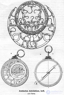
Astrolabe (1208, Persia)
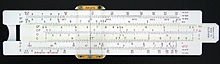
Slide rule
Note: for comparison, selected milestones in the development of digital computing devices are given.
One of the oldest known analog devices is considered to be the Antikythera mechanism — a mechanical device discovered in 1902 on an ancient shipwreck near the Greek island of Antikythera. It dates to approximately 100 BC (possibly as early as 150 BC). It is held at the National Archaeological Museum in Athens.
Astrologers and astronomers used the analog astrolabe from the 4th century BC until the 19th century AD. This instrument was used to determine the positions of stars in the sky and to calculate the length of day and night. A modern descendant of the astrolabe is the planisphere — a movable star chart used for educational purposes.
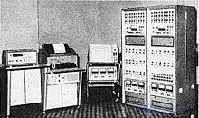
The Polish analog computer “ELWAT”
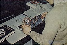
Patch panel of the ELWAT analog computer
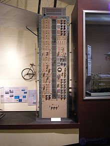
The electronic analog computer MOHAI, built around 1953 by Boeing
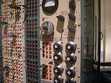
MOHAI close-up
While operating, an analog computer imitates the computation process, with the characteristics representing the numeric data changing continuously over time.
The result of an analog computer's operation is either a graph plotted on paper or on an oscilloscope screen, or an electrical signal used to control a process or the operation of a mechanism.
These computers are ideally suited for automatic control of production processes because they react instantly to various changes in the input data. However, their overall operating speed is low, since the computations largely rely on transient processes in reactive components and are also limited by the frequency bandwidth and load capacity of the operational amplifiers. Computers of this kind were widely used in scientific research — for example, in experiments where inexpensive electrical or mechanical devices are able to model the situation under study.
In a number of cases, analog computers make it possible to solve problems with less concern for computational accuracy than when writing a program for a digital computer. For example, electronic analog computers can readily handle problems that require solving differential equations, integration or differentiation. Specialized circuits and modules, usually built around operational amplifiers, are used for each of these operations. Integration is also easily implemented on hydraulic analog machines.
See: Analog functional block
All the functional blocks of analog computers can be divided into a number of groups:
General-purpose analog computers, as a rule, include:
also used are:
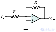
Diagram of a scaling element, also acting as an inverter when k=1
 and the input quantity
  are related by the dependence:
 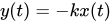 It is used when, in implementing the block diagram of a model on an analog computer, it is necessary to multiply by a constant coefficient
  . A summing block can be used as a scaling element, in which
  and
and  , and the output voltage is given by the dependence:
 .
.
Storage device
See: Sample-and-hold circuit
Figure of merit of an analog computer — a generalized characteristic of an analog computer, calculated using the formula:
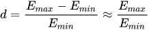 ,
,
where  — the maximum possible value of the machine variable,
  — the lower limit of the possible value of the machine variable. The limits are, as a rule, determined experimentally. The numerical value of depends on the noise level, the errors of the analog functional blocks, and the accuracy of the measuring instrumentation used. The figure of merit of powerful analog computers exceeds
  .
.
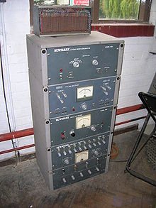
The analog computer “Newmark”, built in 1960. It consists of five units and was used for computing differential equations. It is now held at the Cambridge Museum of Technology
All analog computers can be divided into two main groups:
Mechanical analog computer
An analog computer in which the machine variables are reproduced by mechanical displacements. When solving problems on an analog computer of this type, in addition to scaling the variables, it is necessary to carry out a structural strength analysis and to calculate backlash. The advantages of mechanical analog computers are high reliability and reversibility, which makes it possible to reproduce both direct and inverse mathematical operations. The disadvantages of this type of analog computer are high cost, difficulty of manufacture, large dimensions and weight, and also a low utilization efficiency of the individual computing units. Mechanical analog computers are used in building highly reliable computing devices .
The general name for flow-based (pneumatic and hydraulic) devices intended for computation and similar tasks is pneumonics (see Fluidic logic) .
Pneumatic analog computer
An analog computer in which the variables are represented by air (gas) pressure values at various points of a specially built network. The elements of such an analog computer are throttles, capacitances and diaphragms. The throttles act as resistances and can be fixed, variable, nonlinear or adjustable. The pneumatic capacitances are sealed or through-flow chambers in which the pressure rises as they fill, owing to the compressibility of air. Diaphragms are used to convert air pressure. A pneumatic analog computer may include amplifiers, adders, integrators, function generators and multiplying units, connected to one another by fittings and hoses. Pneumatic analog computers are inferior in speed to electronic ones. On average, the moving elements of such an analog computer have a response time of about a tenth of a millisecond, and can therefore pass frequencies on the order of 10 kHz. Such analog computers are characterized by significant errors, and are therefore used where other types of computing machines cannot be used: in explosive environments, in environments with high temperatures, in automatic chemical-production systems. Because of their low cost and high reliability, such analog computers are also used in metallurgy, heat and power engineering, the gas industry, and so on.
In the 1960s they were developed as a means of achieving discrete computation with high radiation resistance. Elements were developed that perform the basic logical operations and memory elements with no moving mechanical parts.
Such elements are very durable, since they have practically no moving parts and, as a result, nothing to break. If the channels become clogged, the logic matrices are easily disassembled and flushed. A pneumatic computer runs off an industrial compressed-air network. The logic matrices are easily stamped out of thermoplastic on injection-molding machines. For special cases the matrix can be made of refractory ceramic, or cast from iron or another alloy.
Today pneumatic computers are used in industries where increased vibration resistance is required, where operation is needed across a very wide temperature range, or where control of pneumatic power devices is required. In the latter case, there is no need for converters that turn an electrical signal into displacement (electro-pneumatic converter + positioner). These are robots and automation systems working in metallurgy and in mining. There are known cases of their use in controlling elements of aircraft engines, the automation of rocket systems, and the power actuators of helicopters and airplanes.
There is also an entire category of production facilities, units and installations where the use of electricity, even at the lowest voltages, is highly undesirable. This includes organic chemistry, oil refineries, and underground coal and ore mining. They make extensive use of pneumatic automation.
Hydraulic analog computers
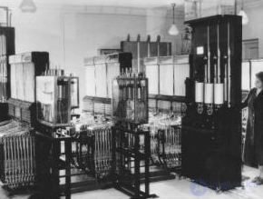
A three-dimensional experimental water integrator by Lukyanov
V. S. Lukyanov proposed the principle of hydraulic analogies in 1934 and in 1936 built the first “water integrator” — a device intended for solving differential equations, whose operation is based on the flow of water. Later, devices of this kind were used at dozens of organizations and remained in use until the mid-1980s .
The first units were rather experimental, made of tin and glass tubes, and each could only be used to solve a single problem.
In 1941 Lukyanov built a water integrator of modular design, which made it possible to assemble a machine for solving a variety of problems.
In 1949 William Phillips built the hydraulic computer MONIAC.
In 1949—1955, at the NIISCHETMASH institute, an integrator was developed in the form of standard unified units. In 1955, at the Ryazan Calculating and Analytical Machines Plant, series production began of integrators under the factory brand “IGL” (Integrator, Hydraulic, of the Lukyanov system).
Two of Lukyanov's water integrators are currently held at the Polytechnic Museum .
Electrical analog computers
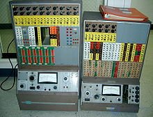
An analog computer with patch panels
These are analog computers in which the variables are represented by DC electrical voltage. They became widespread owing to their high reliability, speed, and convenience of operation and of obtaining results.
Combined analog computers
Not to be confused with Hybrid computer.
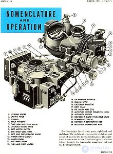
A manual page describing the precision analog aiming mechanism of the American “Norden” bombsight for World War II bombers
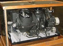
The “Norden” analog bombsight, assembled
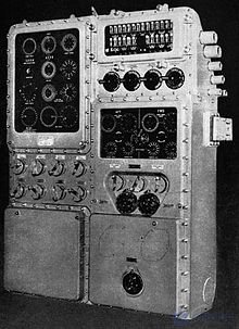
US Navy Mk III Torpedo Data Computer, an analog computer for torpedo fire control. It was used on American submarines during World War II
Electromechanical analog computers
An example of a combined analog computer is the electromechanical analog computer, in which the machine variables are mechanical (usually an angle of rotation) and electrical (usually a voltage) quantities. Specific to this type of analog computer are rotary transformers (synchros) and tachogenerators. Analog computers of this type are less reliable than mechanical ones, owing to the presence of sliding contacts.
Matrix-type analog computer
A matrix-type analog computer (group analog machine) — an analog machine in which individual, simplest computing blocks are rigidly connected into identical standard groups. It is used mainly for modeling differential equations. The problem must first be reduced to an equivalent system of first-order differential equations. Each standard group of computing elements is used to model one equation. A matrix-type analog computer requires a certain scaling process, in which the coefficient values of one matrix column must be of the same order of magnitude. Setting up problems on such analog computers comes down to setting the coefficients and initial conditions. The disadvantage of this type of analog computer is the low utilization efficiency of individual blocks. Mechanical analog computers mainly belong to this type .
Structural-type analog computer
A structural operational analog machine, in which the simplest computing blocks are connected to one another in accordance with the mathematical operations of the equation being solved. Used for mathematical modeling.
Fast (repetitive-operation) analog computer
An analog computer with periodization, with repetition of the solution — an analog computer in which the stages of solving problems are automatically repeated by means of a switching system. The limit of the repetition frequency is determined by the frequency characteristics of the solving elements. The single-shot computing elements of an analog computer (operational amplifiers, function generators, etc.) are suitable for use in a repetitive-operation analog computer. Such analog computers use integrators with a small time constant. The design of high-speed analog computers is more complex than that of single-shot analog computers, since special circuits are needed for discharging capacitors at the end of a cycle and circuits for automatically entering the initial values at the start of each computing cycle. The greatest advantage of an analog computer of this type is the ability to observe the change in the result as a function of the parameters in real time. High-speed analog computers are used for the approximate determination of the transfer function of a physical system from a family of its transient responses, for solving boundary-value problems, computing the Fourier integral, and correlation analysis.
Slow analog computer
A single-shot analog computer in which integrators with relatively large time constants are used. Solving typical problems on such analog computers takes from a few seconds to several minutes. In this case, the result of changing the parameters can only be recorded after all computing cycles have been completed.
Iterative analog computer
See: Iterator
An analog computer that carries out the process of solving a problem by an iterative method over a certain number of iterations. The specific nature of such an analog computer makes it possible to control the course of the computation at specified moments in time. For example, it is possible to process values from the outputs of integrators and to pass information from one cycle to another depending on conditions .
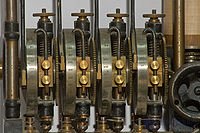
Indicator of a cam-type analog computer
Analog electronic computers are based on setting the physical characteristics of their components. This is usually done by switching individual elements into or out of the circuits that connect these elements by wires, and by changing the parameter values of variable resistors, capacitors and inductors in the circuits.
An automobile automatic transmission is an example of a hydromechanical analog computer, in which, as the torque changes, the fluid in the hydraulic drive changes pressure, making it possible to obtain the required final gear ratio.
Before the advent of powerful and reliable digital equipment, analog computers were widely used in aviation and rocket technology, for the real-time processing of various information and the subsequent generation of control signals in autopilots and other, more complex flight automatic-control systems, or other specialized processes.
In addition to technical applications (automatic transmissions, music synthesizers), analog computers are used to solve specific computational problems of a practical nature. For example, the cam-type mechanical analog computer shown in the photo was used in locomotive engineering to approximate fourth-order curves by means of Fourier transforms.
Mechanical computers were used on early space flights and output information by means of the displacement of a surface indicator. From the first crewed space flight until 2002, every crewed Soviet and Russian spacecraft of the Vostok, Voskhod and Soyuz series was equipped with the “Globus” instrument, which showed the Earth's motion via the displacement of a miniature globe and displayed latitude and longitude data.
In military technology, another name has historically developed for analog computing devices used for artillery fire control, high-altitude bombing and other military tasks requiring complex calculations — this is the fire-control computer (“counting-and-solving instrument”). An example is an anti-aircraft fire-control instrument.
Analog technology is of interest to the military for two features: it is extremely fast, and under conditions of interference the machine's operability is restored as soon as the interference disappears.
Today, analog computers have given way to digital technologies, and to automation and signal-processing systems built around certain FPGA chips for “mixed” digital and analog signals.
From a mathematical point of view, the similarity between linear mechanical components, such as springs and dampers (viscous-fluid dampers), and electrical components, such as capacitors, inductors and resistors, is striking. They can be modeled using equations of the same form.
However, the difference between these systems is what makes analog computation useful. If one considers a simple mass-spring system, building the physical system would require creating or modifying springs and masses. These would then need to be attached to one another and to an appropriate anchor, test equipment with the appropriate range of input signals assembled, and finally the measurements taken. In more complex cases, such as suspensions for racing cars, experimental construction, modification and testing are all at once complex and expensive.
The electrical equivalent can be built using a handful of operational amplifiers (op-amps) and a few passive linear components; all measurements can be taken directly with an oscilloscope. In the circuit, the (simulated) spring stiffness, for example, can be changed by adjusting the integrator's parameters. The electrical system is an analog of the physical system, hence the name, but it is less costly to build, generally safer, and usually much easier to modify.
In addition, the electronic circuit can usually operate at higher frequencies than the system being modeled. This allows the simulation to run faster than real time (which, in some cases, can last hours, weeks, or longer). Experienced users of electronic analog computers say that they offer comparatively thorough control of, and insight into, the problem compared with digital simulation.
A drawback of the mechanical-electrical analogy is that electronics are limited in the range over which variables can change, because of the fixed supply voltage. Consequently, each problem must be scaled to match its parameters and dimensions — for example, the expected magnitudes of velocity and the position of a spring pendulum. Problems that are scaled incorrectly may suffer from a higher noise level. Digital floating-point computation has an enormous dynamic range, but it too can suffer from inaccuracy if tiny differences between huge values lead to numerical instability.
These electrical circuits can also easily perform a wide variety of simulations. For example, voltage can model water pressure, and electric current can model the flow rate in cubic meters per second. An integrator can provide the total accumulated volume of fluid, using an input current proportional to the (possibly varying) flow rate.
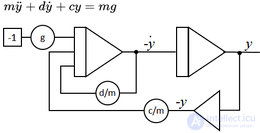
Analog circuit for the dynamics of a mass-spring system (without scale factors)


Damped motion of a mass-spring system
Analog computers are particularly well suited to representing situations described by differential equations. They were sometimes used when a system of differential equations was very difficult to solve by conventional means. As a simple example, the dynamics of a mass-spring system can be described by the equation  , [ citation needed ] with
  as the vertical position of the mass
  ,
,  the damping coefficient,
  the spring constant and
  Earth's gravitational acceleration. For analog computation the equation is programmed as -
  . The equivalent analog circuit consists of two integrators for the state variables
  (velocity) and (position), one inverter, and three potentiometers. The circuit must allow for the fact that both the integrating and summing blocks invert the signal's polarity.
The precision of an analog computer is limited by its computing elements, as well as by the quality of the internal power supply and the electrical connections. The precision of an analog computer's readout was limited mainly by the accuracy of the readout equipment used, typically to three or four significant digits. The precision of a digital computer is limited by its word length; arbitrary-precision arithmetic, although relatively slow, provides whatever practical degree of precision may be required. In most cases, however, the precision of an analog computer is entirely adequate, given the uncertainty in the model's characteristics and its technical parameters.
Many small computers designed for specific calculations are still part of industrial control equipment today, but from the 1950s through the 1970s, general-purpose analog computers were the only systems fast enough for real-time simulation of dynamic systems, especially in the aircraft, military and aerospace fields.
In the 1960s, the leading manufacturer was Electronic Associates of Princeton, New Jersey , with the 231R analog computer (vacuum tubes, 20 integrators), and later the EAI 8800 analog computer (solid-state operational amplifiers, 64 integrators). [31] Its rival was Applied Dynamics of Ann Arbor, Michigan .
Although the underlying technology for analog computers is usually operational amplifiers (also called “DC amplifiers”, because they have no low-frequency cutoff), in the 1960s the French ANALAC computer attempted to use an alternative technology: a medium-frequency carrier and non-dissipative, reversible networks.
In the 1970s, every major company and agency dealing with problems of dynamics had a large analog-computing center, for example:
Electronic analog computers usually have front panels with numerous jacks (single-contact sockets) that let patch cords (flexible wires with plugs at both ends) make the connections that define the problem setup. There are also precision, high-resolution potentiometers (variable resistors) for setting (and, when necessary, changing) scale factors. In addition, there is usually a zero-centered analog needle meter for measuring voltage to moderate accuracy. Stable, accurate voltage sources supply known quantities.
Typical electronic analog computers contain anywhere from a few to a hundred or more operational amplifiers (“op-amps”), so named because they perform mathematical operations. Op-amps are a special type of feedback amplifier with very high gain and a stable input (low and stable offset). They are always used with precision feedback components which, in operation, virtually cancel out the currents coming from the input components. Most of the op-amps in a representative setup are summing amplifiers, which add and subtract analog voltages, delivering the result at their output terminals. In addition, op-amps with capacitive feedback are usually included; these integrate the sum of their inputs over time.
Integration with respect to a variable other than time is almost the exclusive province of mechanical analog integrators; it is almost never done in electronic analog computers. However, given that the solution to the problem does not change over time, time can serve as one of the variables.
Other computing elements include analog multipliers, nonlinear function generators, and analog comparators.
Electrical elements such as inductors and capacitors used in electrical analog computers had to be carefully manufactured to reduce non-ideal effects. For example, when building AC power-network analyzers, one motivation for using higher frequencies in the computer (instead of the actual mains frequency) was that higher-quality inductors could be more easily manufactured. Many general-purpose analog computers avoid the use of inductors altogether, recasting the problem in a form that can be solved using only resistive and capacitive elements, since high-quality capacitors are relatively easy to manufacture.
The use of electrical properties in analog computers means that calculations are usually carried out in real time (or faster), at a speed determined mainly by the frequency response of the operational amplifiers and other computing elements. In the history of electronic analog computers there have been several special high-speed types.
Nonlinear functions and computations can be built with limited precision (three or four digits) by designing function generators — special circuits made of various combinations of resistors and diodes to provide the nonlinearity. As a rule, as the input voltage increases, more diodes conduct.
With temperature compensation, the forward voltage drop across a transistor's base-emitter junction can provide a sufficiently accurate logarithmic or exponential function. Operational amplifiers scale the output voltage so that it can be used with the rest of the computer.
Any physical process that models some computation can be interpreted as an analog computer. Some examples devised to illustrate the concept of analog computation include using a bundle of spaghetti as a model for sorting numbers ; a board, a set of nails and a rubber band as a model for finding the convex hull of a set of points; and strings tied together as a model for finding the shortest path in a network. All of these are described by Dewdney (1984).
Analog computing devices are fast, digital computing devices are more versatile and precise, so the idea is to combine the two approaches for maximum efficiency. An example of such an elementary hybrid device is the hybrid multiplier, in which one input is an analog signal, the other input is a digital signal, and the output is analog. It acts as a digitally updated analog potentiometer. This kind of hybrid technique is used mainly for fast, dedicated real-time computation, where computation time is very critical, in radar signal processing and, generally, for controllers in embedded systems .
In the early 1970s, manufacturers of analog computers tried to link their analog computers to digital ones, in order to get the advantages of both approaches. In such systems, a digital computer controlled the analog computer, providing the initial setup, triggering a series of analog runs, and automatically entering and collecting data. The digital computer could also take part in the calculation itself, by means of analog-to-digital and digital-to-analog converters .
The largest manufacturer of hybrid computers was Electronic Associates. Their model 8900 hybrid computer consisted of a digital computer and one or more analog consoles. These systems were mainly intended for major programs such as Apollo and the Space Shuttle at NASA, or Ariane in Europe, especially during the integration phase, when everything is simulated at first and the simulated parts are gradually replaced by real components. [32]
Only one company was known to offer general commercial computing services on its hybrid computers — CISI of France, in the 1970s.
The best reference material in this field is the 100,000 simulation runs performed for each certification of the Airbus and Concorde automatic landing systems . [33]
After 1980, purely digital computers developed faster and faster and became fast enough to compete with analog computers. One of the keys to the speed of analog computers was their fully parallel computation, but this was also a limitation. The more equations a problem required to solve, the more analog components were needed, even if the problem was not time-critical. “Programming” a problem meant wiring together analog operators; even with a removable patch panel, this was not very versatile. Today there are no longer any large hybrid computers, only hybrid components.
In general, analog computers are limited by non-ideal effects. An analog signal consists of four basic components: DC and AC, magnitude of frequency, and phase. Real-world limits on the range of these characteristics constrain analog computers. Some of these limitations include operational-amplifier offset, finite gain and frequency response, a minimum noise floor , nonlinearities , temperature coefficient, and parasitic effects in semiconductor devices. For commercially available electronic components, the ranges of these aspects of the input and output signals are always indicators of quality .
The Polish electronic analog computer “AKAT-1”
Among analog computing devices, the following can be singled out:
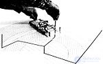 |
The FERMIAC in use
The FERMIAC — an analog computer invented by the physicist Enrico Fermi in 1946 to assist his research. It used the Monte Carlo method to simulate the movement of neutrons in various types of nuclear systems. Given an initial distribution of neutrons, the goal of the simulation is to work out numerous “neutron genealogies”, or models of the behavior of individual neutrons, including every collision, scattering event and nuclear fission. At each step, pseudorandom numbers — “generated” by the settings of the device's drums — were used to decide the neutrons' behavior.
“Iterator” — a specialized analog computer designed to solve linear boundary-value problems for systems of linear differential equations. It was developed at the Institute of Cybernetics of the Academy of Sciences of the Ukrainian SSR in 1962.
“Iterator” solves the boundary-value problem by Newton's iterative method, reducing it to the solution of several differential equations with given initial conditions. This algorithm consists of determining the matrix of first derivatives with respect to the components of the initial-condition vector, and automatically searching for the solution to the boundary-value problem using this matrix. Thanks to the method used, convergence of the iterative process, to within a specified permissible solution error, is achieved in three to four iterations.
In addition to systems of differential equations with constant and variable coefficients of order 2n with linear boundary conditions, “Iterator” solves systems of linear algebraic equations of order n with an arbitrary coefficient matrix.
Specifications
A family of analog computing machines. The name is an abbreviation of the words “model, nonlinear”. They were designed to solve Cauchy problems for ordinary differential equations. The most advanced machine in this line was the “MN-18” — a medium-power analog computer designed to solve, by mathematical-modeling methods, complex dynamic systems described by differential equations of up to the tenth order, either as part of an analog-digital computing complex or on its own. The control circuit allows integrators to be started simultaneously or separately by group, and allows both single-shot problem solving and repeated problem solving. Up to four MN-18 machines can be combined into a single complex.
Specifications
The human brain is the most powerful and efficient “analog device” there is. And although the transmission of nerve impulses relies on discrete signals, the information in the nervous system is not represented digitally. Neurocomputers are analog, hybrid computers (models implemented on digital computers) built from elements that function similarly to brain cells .

Comments