
Lecture

Today we will discuss in detail an important class of machine learning models – linear models. The key difference between our presentation of the material and similar courses in econometrics and statistics is the emphasis on the practical application of linear models to real-world problems (although there will be plenty of math too).
An example of such a problem is the Kaggle Inclass competition on identifying a user on the Internet by their sequence of site visits.
Outline of this article:
We will start our discussion of linear models with linear regression. First of all, we need to specify a model for the dependence of the explained variable  on the explanatory factors, with the dependence function being linear:
 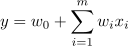 . If we add a dummy dimension
  for each observation, then the linear form can be rewritten a bit more compactly, by moving the intercept
  under the summation:
 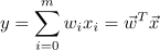 . If we consider the observations-features matrix, in whose rows lie the examples from the dataset, then we need to add a column of ones on the left. Let us specify the model as follows:

where
 – the explained (or target) variable;
 – vector of model parameters (in machine learning these parameters are often called weights);
 – observations and features matrix of dimension
  rows by
  columns (including the dummy column of ones on the left) with full column rank:
  ;
; – a random variable corresponding to the random, unpredictable error of the model.
We can write the expression for each specific observation
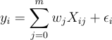
The model is also subject to the following constraints (otherwise it would be some other kind of regression, but definitely not linear):
 ;
; ;
; .
.
An estimate  of the weights
  is called linear if

where  depends only on the observed data and, almost surely, nonlinearly. Since the solution of the problem of finding the optimal weights is precisely a linear estimate, the model is called linear regression. Let us introduce one more definition. An estimate is called unbiased when the expected value of the estimate equals the real, but unknown, value of the parameter being estimated:

One way to compute the values of the model parameters is the least squares method (OLS), which minimizes the mean squared error between the real value of the dependent variable and the prediction produced by the model:
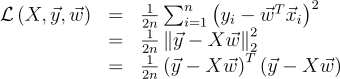
To solve this optimization problem, we need to compute the derivatives with respect to the model parameters, set them equal to zero, and solve the resulting equations for  (matrix differentiation may seem difficult to an unprepared reader; try writing everything out through sums to verify the answer):
Cheat sheet on matrix derivatives
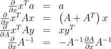

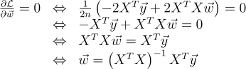
So, keeping in mind all the definitions and conditions described above, we can assert, relying on the Gauss-Markov theorem, that the OLS estimate is the best estimate of the model parameters among all linear and unbiased estimates, that is, the one having the smallest variance.
The reader may well have questions: for example, why do we minimize the mean squared error and not something else. After all, one could minimize the mean absolute value of the residual or something else. The only thing that would happen if we changed the value being minimized is that we would step outside the conditions of the Gauss-Markov theorem, and our estimates would no longer be the best among linear and unbiased ones.
Before we continue, let us take a lyrical digression to illustrate the maximum likelihood method with a simple example.
Once, after school, I noticed that everyone remembers the formula for ethyl alcohol. So I decided to run an experiment: do people remember the simpler formula for methyl alcohol:  . We surveyed 400 people, and it turned out that only 117 people remembered the formula. It is reasonable to assume that the probability that the next person surveyed knows the formula for methyl alcohol is
  . Let us show that this intuitively obvious estimate is not just good, but is in fact the maximum likelihood estimate.
Let us figure out where this estimate comes from, and for that let us recall the definition of the Bernoulli distribution: a random variable has a Bernoulli distribution if it takes only two values ( and
and  with probabilities
  and
and  respectively) and has the following probability distribution function:

It looks like this distribution is what we need, and the distribution parameter is precisely the estimate of the probability that a person knows the formula for methyl alcohol. We ran  independentexperiments, and denote their outcomes as
  . Let us write the likelihood of our data (observations), that is, the probability of observing 117 realizations of the random variable
  and 283 realizations of
  :
:

Next we will maximize this expression with respect to , and most often this is done not with the likelihood  itself, but with its logarithm (applying a monotonic transformation will not change the solution, but will simplify the calculations):


Now we want to find the value of that maximizes the likelihood; to do this we will take the derivative with respect to , set it equal to zero, and solve the resulting equation:


It turns out that our intuitive estimate is exactly the maximum likelihood estimate. Let us now apply the same reasoning to the linear regression problem and try to find out what lies behind the mean squared error. To do this, we will need to look at linear regression from a probabilistic point of view. The model, naturally, remains the same:
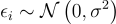
but now we will assume that the random errors are drawn from a centered normal distribution:
Let us rewrite the model in this new light:

Since the examples are drawn independently (the errors are uncorrelated – one of the conditions of the Gauss-Markov theorem), the full likelihood of the data will look like the product of the density functions  . Let us consider the log-likelihood, which will let us move from a product to a sum:
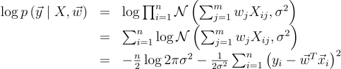
We want to find the maximum likelihood hypothesis, i.e. we need to maximize the expression  , which is the same as maximizing its logarithm. Note that when maximizing a function with respect to some parameter, all terms that do not depend on that parameter can be discarded:
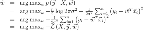
Thus, we have seen that maximizing the likelihood of the data is the same as minimizing the mean squared error (given that the assumptions stated above hold). It turns out that this particular cost function is precisely a consequence of the error being normally distributed, and not distributed in some other way.
Let us talk a bit about the properties of the prediction error of linear regression (in principle, this reasoning holds for all machine learning algorithms). In light of the previous section, we found that:
 and a random error :
  ;
; ;
; by a linear function of the regressors
  , which, in turn, is a point estimate of the function
  in function space (more precisely, we have restricted the function space to the parametric family of linear functions), i.e. a random variable that has a mean value and a variance.
Then the error at point  decomposes as follows:
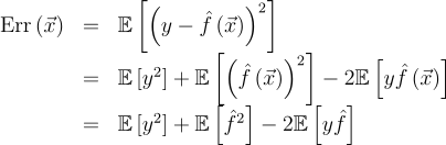
For clarity, let us omit the notation of the functions' argument. Let us consider each term separately; the first two are easy to expand using the formula  :
:
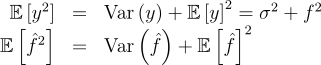
Explanations:
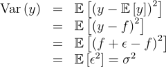

And now the last term of the sum. We recall that the error and the target variable are independent of each other:
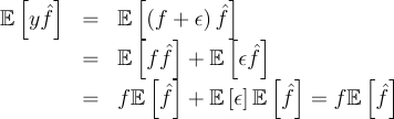
Finally, let us put it all together:
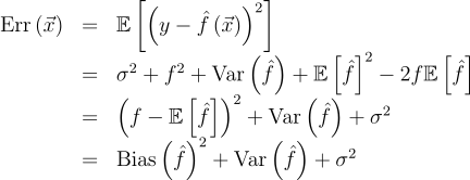
So, we have reached the goal of all the calculations described above; the final formula tells us that the prediction error of any model of the form is made up of:
 – the average error over all possible datasets;
 – the variability of the error, i.e. how much the error will differ if the model is trained on different datasets;
 .
.
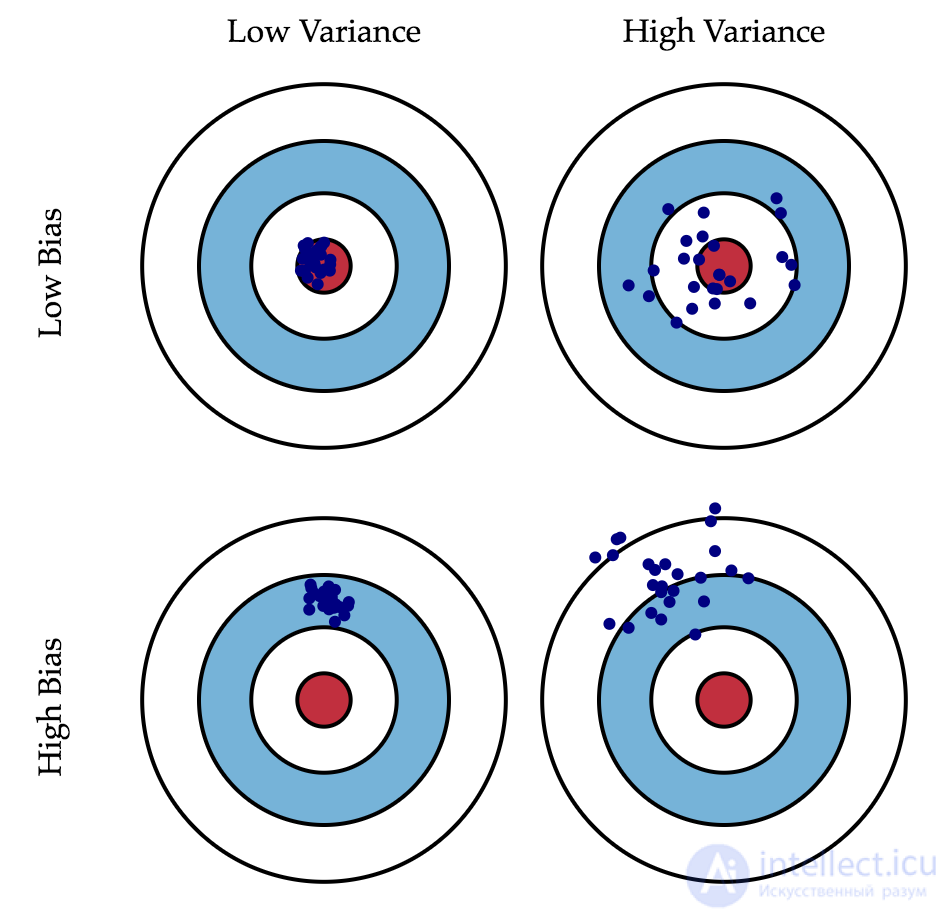
While we can do nothing about the last term, we can somehow influence the first two. Ideally, of course, we would want to reduce both of these terms to zero (the upper left square of the figure), but in practice we often have to balance between biased and unstable estimates (high variance).
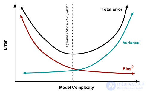
As a rule, as model complexity increases (for example, as the number of free parameters increases), the variance (spread) of the estimate increases, but the bias decreases. Because the training dataset is completely memorized instead of being generalized, small changes lead to unexpected results (overfitting). If, on the other hand, the model is weak, it is unable to learn the underlying pattern, and as a result it learns something else, biased relative to the correct solution.
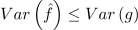
The Gauss-Markov theorem states precisely that the OLS estimate of the parameters of a linear model is the best in the class of unbiased linear estimates, that is, it has the smallest variance. This means that if there exists some other unbiased model  that is also in the class of linear models, we can be sure that
  .
.
Sometimes there are situations where we deliberately increase the bias of a model for the sake of its stability, i.e. in order to reduce the variance of the model . One of the conditions of the Gauss-Markov theorem is that the matrix has full column rank. Otherwise, the OLS solution  does not exist, since the inverse matrix
  would not exist. In other words, the matrix
  would be singular, or degenerate. Such a problem is called ill-posed. The problem needs to be corrected, namely, the matrix needs to be made non-degenerate, or regular (which is precisely why this process is called regularization). More often, in data we can observe so-called multicollinearity — when two or more features are strongly correlated, which in the matrix shows up as an "almost" linear dependence between columns. For example, in the problem of predicting an apartment's price from its parameters, the features "area including the balcony" and "area excluding the balcony" would have an "almost" linear dependence. Formally, for such data the matrix would be invertible, but due to multicollinearity some eigenvalues of the matrix will be close to zero, and extremely large eigenvalues will appear in the inverse matrix
  , since the eigenvalues of the inverse matrix – are
  . The result of this instability in the eigenvalues will be an unstable estimate of the model parameters, i.e. adding a new observation to the training dataset will lead to a completely different solution. You can find illustrations of the growth of the coefficients in one of our previous posts. One method of regularization is Tikhonov regularization, which in general form looks like adding a new term to the mean squared error:

The Tikhonov matrix is often expressed as the product of some number and the identity matrix:  . In this case, the problem of minimizing the mean squared error becomes a problem with a constraint on the
  norm. If we differentiate the new cost function with respect to the model parameters, set the resulting function equal to zero, and solve for , we obtain the exact solution to the problem.

Such a regression is called ridge regression. And the ridge is precisely the diagonal matrix that we add to the matrix , which results in a matrix that is guaranteed to be regular.

This solution reduces variance, but becomes biased, since the norm of the parameter vector is also minimized, which forces the solution to shift toward zero. In the figure below, the OLS solution is located at the intersection of the white dashed lines. The blue dots denote various ridge regression solutions. It can be seen that as the regularization parameter  increases, the solution shifts toward zero.
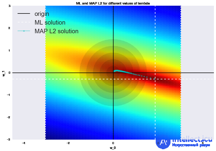
We recommend checking our previous post for an example of how regularization deals with the problem of multicollinearity, as well as to refresh your memory of a few more interpretations of regularization.
The main idea of a linear classifier is that the feature space can be divided by a hyperplane into two half-spaces, in each of which one of the two values of the target class is predicted.
If this can be done without errors, the training sample is called linearly separable.
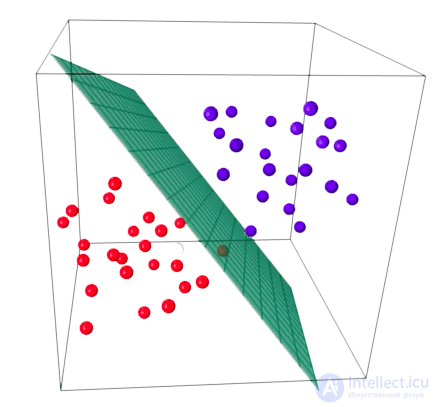
We are already familiar with linear regression and the least squares method. Let us consider the binary classification problem, where we denote the labels of the target class as "+1" (positive examples) and "-1" (negative examples).
One of the simplest linear classifiers is obtained from regression in the following way:

where
– the feature vector of the example (together with the one); – the weights of the linear model (together with the bias ); – the "signum" function, which returns the sign of its argument;
 – the classifier's response on example .
Logistic regression is a special case of a linear classifier, but it has a nice "ability" – to predict the probability  of assigning example
  to class "+":

Predicting not just the answer ("+1" or "-1"), but specifically the probability of belonging to class "+1", is a very important business requirement in many problems. For example, in the credit scoring problem, where logistic regression is traditionally used, the probability of loan default is often predicted (). Clients who have applied for a loan are sorted by this predicted probability (in descending order), producing a scorecard — essentially a ranking of clients from bad to good. A toy example of such a scorecard is given below.
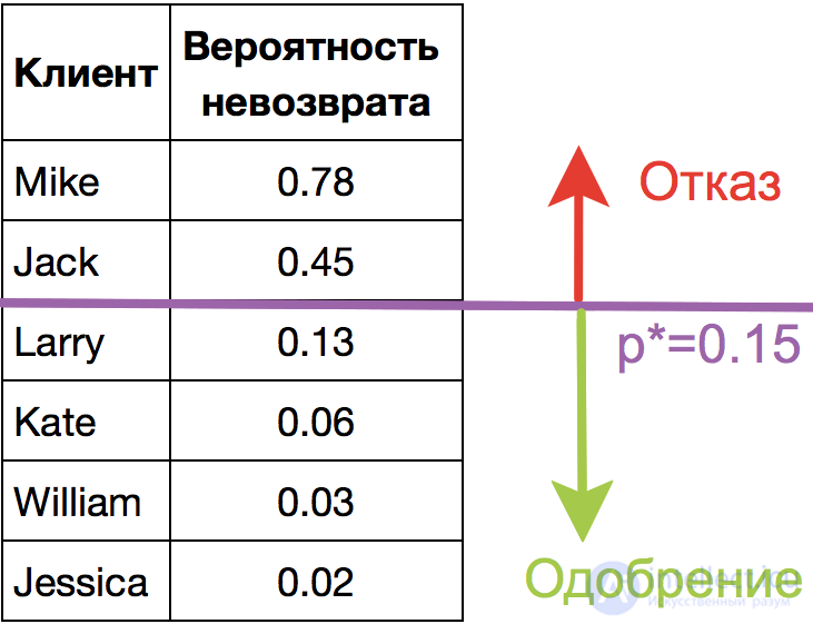
The bank chooses for itself a threshold  for the predicted probability of loan default (in the picture –
  ), and starting from this value it no longer issues the loan. Moreover, one can multiply the predicted probability by the amount issued and obtain the expected loss from the client, which is also a good business metric (Scoring specialists are welcome to correct this in the comments, but that's roughly the main idea).
So, we want to predict the probability  , and so far we know how to build a linear prediction using OLS:
  . How can we transform the resulting value into a probability, whose bounds are [0, 1]? Obviously, for this we need some function
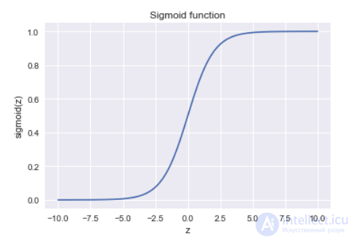
  In the logistic regression model, a specific function is used for this:
 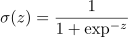 . And now let us figure out what the reasoning behind this is.
Let us denote  as the probability of the event occurring. Then the odds ratio
  is defined from
  , and this — is the ratio of the probability that the event will occur to the probability that it will not. Obviously, the probability and the odds ratio carry the same information. But while ranges from 0 to 1, ranges from 0 to
  .
.
If we compute the logarithm (which is called the log-odds, or logarithm of the odds ratio), it is easy to see that  . It is exactly this that we will predict using OLS.
Let us see how logistic regression makes the prediction  (for now let us assume that we somehow obtained the weights (i.e. trained the model); later we will figure out exactly how).
Step 1. Compute the value  . (the equation
  defines a hyperplane that separates the examples into 2 classes);
Step 2. Compute the log-odds:  .
.
Step 3. Having a prediction of the odds of belonging to class "+" –  , compute using a simple relationship:

On the right-hand side, we obtained precisely the sigmoid function.
So, logistic regression predicts the probability of assigning an example to class "+" (given that we know its features and the model's weights) as the sigmoid transformation of the linear combination of the model's weight vector and the example's feature vector:

The next question is: how is the model trained? Here we again turn to the maximum likelihood principle.
Now let us see how the optimization problem solved by logistic regression follows from the maximum likelihood principle, namely – the minimization of the logistic loss function.
We have just seen that logistic regression models the probability of assigning an example to class "+" as

Then for class "-" the analogous probability is:

Both of these expressions can be cleverly combined into one (watch my hands – make sure I'm not tricking you):

The expression  is called the margin (margin) of classification on object (not to be confused with the gap (also called margin), which is more often discussed in the context of SVM). If it is non-negative, the model does not make a mistake on object ; if it is negative, this means that the class for was predicted incorrectly.
Note that the margin is defined specifically for objects of the training set, for which the real labels of the target class  are known.
To understand why we drew these conclusions, let us turn to the geometric interpretation of the linear classifier. You can read more about this in the materials by Evgeny Sokolov.
I recommend solving an almost classic problem from an introductory linear algebra course: find the distance from a point with radius-vector  to a plane given by the equation
Answer
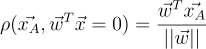
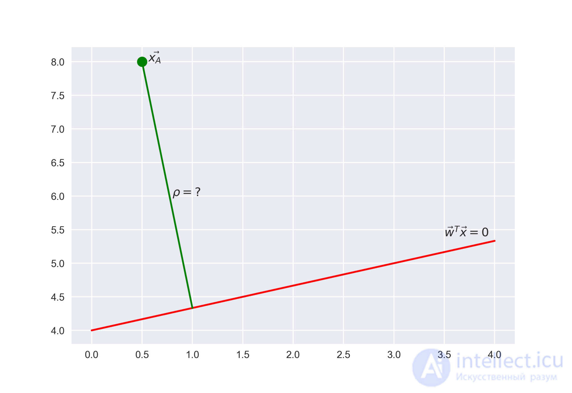
Once we obtain (or look at) the answer, we will understand that the larger the absolute value of the expression  , the farther the point is from the plane
This means that the expression – is a kind of "confidence" of the model in classifying the object :
 .
. .
. and
and  .
.
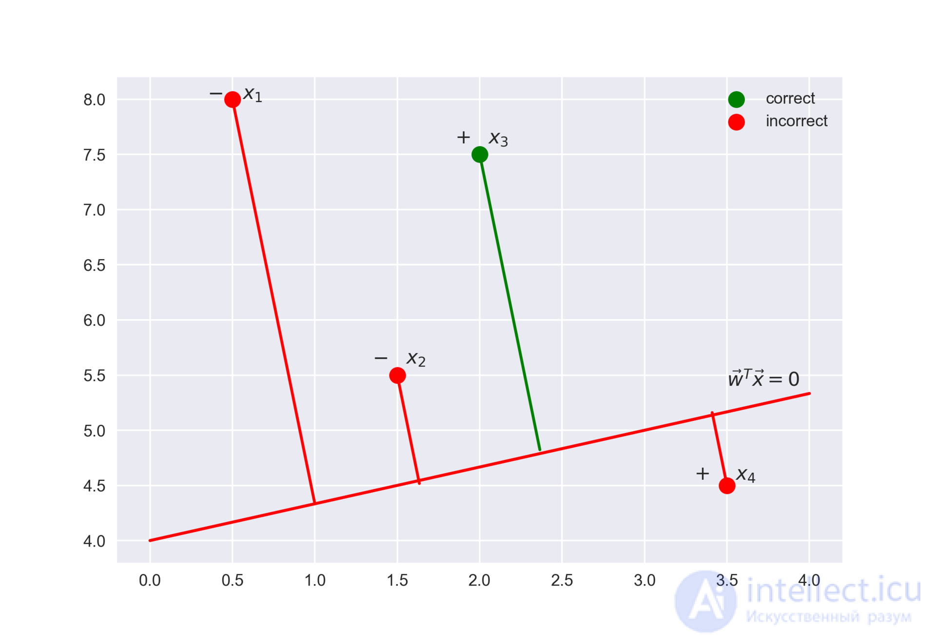
Now let us write out the likelihood of the sample, namely, the probability of observing the given vector  for the sample . We make a strong assumption: the objects arrive independently, from the same distribution (i.i.d.). Then

where  – is the length of the sample (the number of rows).
As usual, let us take the logarithm of this expression (a sum is much easier to optimize than a product):
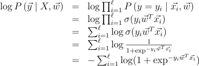
That is, in this case the maximum likelihood principle leads to minimizing the expression

This is the logistic loss function, summed over all objects of the training set.
Let us look at this new function as a function of the margin:  . Let us plot its graph, along with the graph of the 1/0 loss function (zero-one loss), which simply penalizes the model by 1 for an error on each object (negative margin):
  .
.
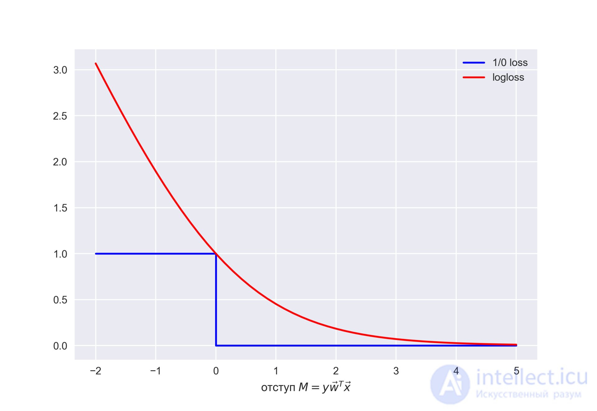
The picture reflects the general idea that in the classification problem, unable to directly minimize the number of errors (at least, this cannot be done with gradient methods – the derivative of the 1/0 loss function at zero goes to infinity), we minimize some upper bound of it. In this case, this is the logistic loss function (where the logarithm is binary, but that is not essential), and the following holds
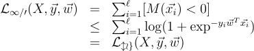
where  – is simply the number of errors of logistic regression with weights on the sample
  .
.
That is, by decreasing the upper bound  on the number of classification errors, we thus hope to decrease the number of errors itself as well.
-regularization of logistic loss
L2-regularization of logistic regression works in almost the same way as for ridge regression. Instead of the functional  , the following is minimized:

In the case of logistic regression, it is customary to introduce the inverse regularization coefficient  . And then the solution to the problem will be

Next, let us look at an example that will let us intuitively understand one of the meanings of regularization.
In article 1 we already gave an example of how polynomial features allow linear models to build nonlinear separating surfaces. Let us show this with pictures.
Let us see how regularization affects classification quality on the microchip testing dataset from Andrew Ng's machine learning course.
We will use logistic regression with polynomial features and vary the regularization parameter C.
First, let us see how regularization affects the classifier's separating boundary, and intuitively recognize overfitting and underfitting.
Then, let us numerically find a near-optimal regularization parameter using cross-validation and grid search (GridSearch).
Importing the libraries
from __future__ import division, print_function
# turn off all the Anaconda warnings
import warnings
warnings.filterwarnings('ignore')
%matplotlib inline
from matplotlib import pyplot as plt
import seaborn as sns

import numpy as np
import pandas as pd
from sklearn.preprocessing import PolynomialFeatures
from sklearn.linear_model import LogisticRegression, LogisticRegressionCV
from sklearn.model_selection import cross_val_score, StratifiedKFold
from sklearn.model_selection import GridSearchCV
Let us load the data using the read_csv method of the pandas library. In this dataset, for 118 microchips (objects) the results of two quality control tests (two numeric features) are given, along with whether the microchip was put into production. The features have already been centered, that is, the column means have been subtracted from all values. Thus, the "average" microchip corresponds to zero values of the test results.
Loading the data
data = pd.read_csv('../../data/microchip_tests.txt',
header=None, names = ('test1','test2','released'))
# dataset info
data.info()
RangeIndex: 118 entries, 0 to 117
Data columns (total 3 columns):
test1 118 non-null float64
test2 118 non-null float64
released 118 non-null int64
dtypes: float64(2), int64(1)
memory usage: 2.8 KB
Let us look at the first and last 5 rows.
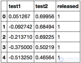
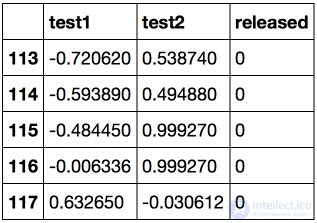
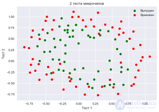
Let us save the training set and the target class labels in separate NumPy arrays. Let us plot the data. Red corresponds to defective chips, green – to normal ones.
Code
X = data.ix[:,:2].values
y = data.ix[:,2].values
plt.scatter(X[y == 1, 0], X[y == 1, 1], c='green', label='Passed')
plt.scatter(X[y == 0, 0], X[y == 0, 1], c='red', label='Defective')
plt.xlabel("Test 1")
plt.ylabel("Test 2")
plt.title('2 microchip tests')
plt.legend();
Let's define a function to display the classifier's separating curve
Code
def plot_boundary(clf, X, y, grid_step=.01, poly_featurizer=None):
x_min, x_max = X[:, 0].min() - .1, X[:, 0].max() + .1
y_min, y_max = X[:, 1].min() - .1, X[:, 1].max() + .1
xx, yy = np.meshgrid(np.arange(x_min, x_max, grid_step),
np.arange(y_min, y_max, grid_step))

# assign a color to each point of the grid [x_min, m_max]x[y_min, y_max]
# in accordance with its class
Z = clf.predict(poly_featurizer.transform(np.c_[xx.ravel(), yy.ravel()]))
Z = Z.reshape(xx.shape)
plt.contour(xx, yy, Z, cmap=plt.cm.Paired)
We call polynomial features up to degree  for two variables and the following:

For example, for  these will be the following features:

If you draw Pascal's triangle, you can figure out how many such features there will be for  and in general for any .
Simply put, there are exponentially many such features, and building, say, polynomial features of degree 10 for 100 features can turn out to be costly (and, moreover, unnecessary).
Let's create an sklearn object that will add polynomial features up to degree 7 to the matrix
продолжение следует...
Часть 1 4. Linear Models for Classification and Regression
Часть 2 4. Where logistic regression is good and where it is

Comments