
Lecture
Hello everyone! It's time to expand our algorithmic arsenal.
Today we'll thoroughly break down one of the most popular and widely used machine learning algorithms in practice — gradient boosting. Where boosting's roots come from and what really happens under the hood of the algorithm — in our colorful journey into the world of boosting, below the cut.
UPD: the course is now available in English under the mlcourse.ai brand, with articles on Medium, and materials on Kaggle (Dataset) and on GitHub.
A video recording of the lecture based on this article, from the second run of the open course (September–November 2017).
List of articles in the series
Plan of this article:
Most people involved in data analysis have heard about boosting at least once. This algorithm is part of the everyday "gentleman's set" of models worth trying on any given task. Xgboost is often associated with the standard recipe for winning ML competitions, giving rise to the meme about "stacking xgboosts". Boosting is also an important part of most search engines, sometimes even serving as their calling card. For general knowledge, let's take a look at how boosting appeared and developed.
It all started with the question of whether it's possible to get one strong model from a large number of relatively weak and simple models. By weak models we don't just mean small and simple models like decision trees as opposed to more "strong" models, such as neural networks. In our case, weak models are arbitrary machine learning algorithms whose accuracy may be only slightly better than random guessing.
An affirmative mathematical answer to this question was found fairly quickly, which in itself was an important theoretical result (a rarity in ML). However, it took several years before workable algorithms and Adaboost appeared. Their general approach consisted of greedily building a linear combination of simple models (base algorithms) by reweighting the input data. Each subsequent model (usually a decision tree) was built in such a way as to give greater weight and preference to previously incorrectly predicted observations.
A bit more about Adaboost
Properly, we should have followed the example of most other machine learning courses and carefully examined its predecessor — Adaboost — before gradient boosting. However, we decided to jump straight to the most interesting part, since Adaboost ended up merging with GBM anyway once it became clear that it's simply a special case of it.
The algorithm itself has a very illustrative visual interpretation of the intuition behind weighting observations. Let's consider a toy classification example, in which on each Adaboost iteration we'll try to split the data with a depth-1 tree (the so-called "stump"). On the first two iterations we'll see the following picture:
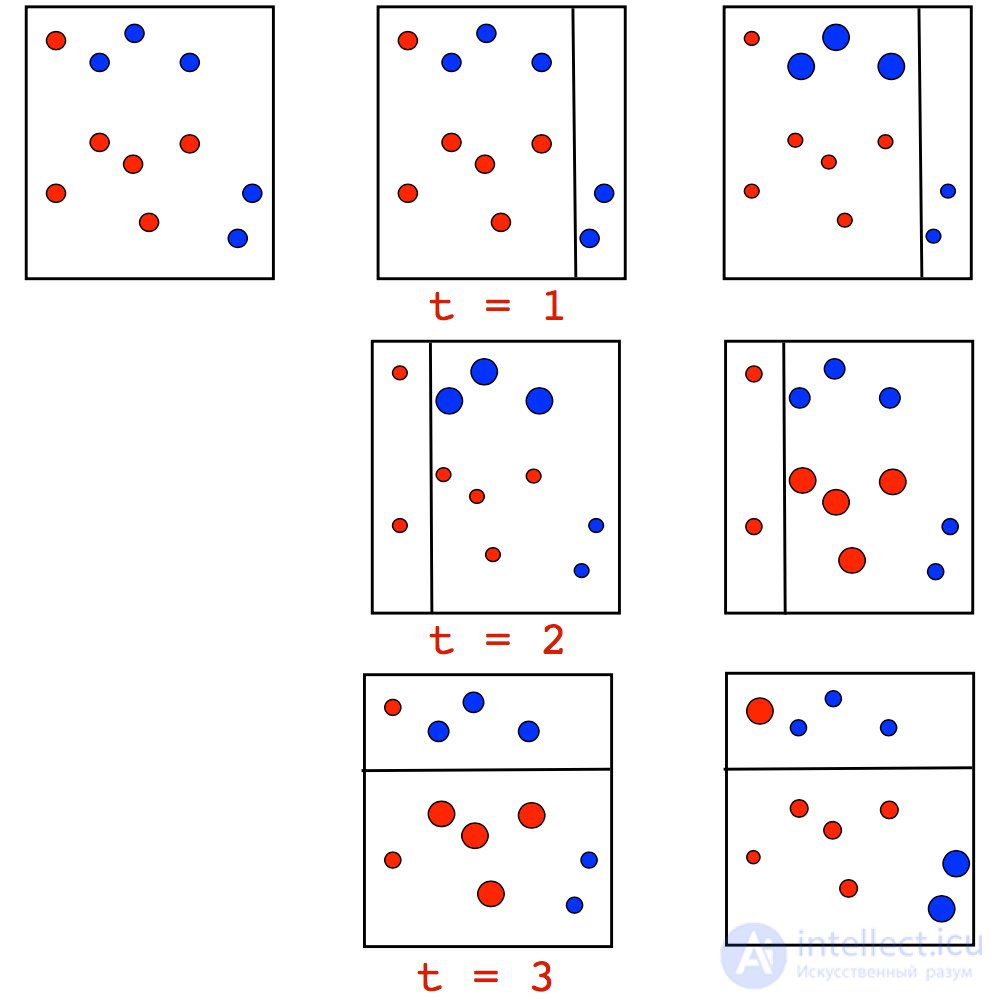
The size of the point corresponds to the weight it received for an incorrect prediction. And we can see how these weights grow with each iteration — the stumps can't handle such a task on their own. However, once we perform a weighted vote of the previously built stumps, we get the split we're looking for:
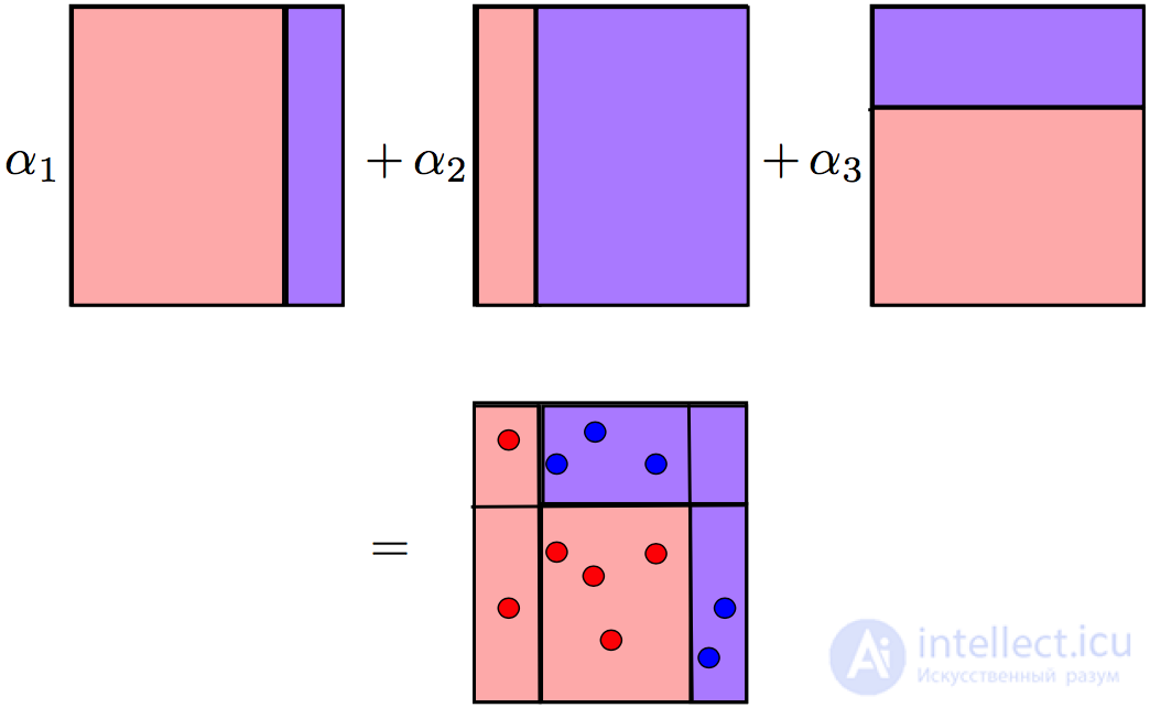
A more detailed example of Adaboost at work, in which over a series of iterations you can see a gradual increase of the points, especially at the boundary between classes:
Adaboost worked well, but because there were few justifications for how the algorithm and its add-ons worked, a full spectrum of speculation arose around them: some considered it a super-algorithm and a magic bullet, others were skeptical and shared the view that it was a barely applicable approach with severe overfitting. This was especially true regarding its applicability to data with strong outliers, to which Adaboost turned out to be unstable. Fortunately, when the professors of the Stanford Statistics Department, who had already given the world Lasso, Elastic Net, and Random Forest, took up the matter, in 1999 Jerome Friedman came up with a generalization of the boosting algorithms — gradient boosting, aka Gradient Boosting (Machine), aka GBM. With this work, Friedman immediately laid a statistical foundation for creating many algorithms, providing a general approach to boosting as optimization in a functional space.
Stanford's legacy
In general, the team at the Stanford Statistics Department is behind CART, bootstrap, and many other things, having already put their names into future statistics textbooks in advance. By and large, a significant part of our everyday toolkit appeared right there, and who knows what else will appear. Or has already appeared but hasn't yet found sufficient adoption (like, for example, glinternet).
There aren't many video recordings with Friedman himself. However, there is a very interesting interview with him about the creation of CART, and in general about how statistical problems (which we would now classify as data analysis and data science) were solved 40+ years ago:
From the series on the educational history of data analysis, there's also a lecture from Hastie with a retrospective on data analysis from one of the people involved in creating the methods we use every day:
Essentially, there was a shift from engineering-algorithmic exploration in building algorithms (so characteristic of ML) to a full-fledged methodology for how to build and study such algorithms. From the point of view of the mathematical substance, at first glance not much changed: we still add (boost) weak algorithms, growing our ensemble with gradual improvements in the areas of the data where previous models "fell short". But when building the next simple model, it's not simply built on reweighted observations, but in such a way as to best approximate the overall gradient of the objective function. On a conceptual level, this opened up a lot of room for imagination and extensions.
Gradient boosting didn't take its place in the "gentleman's set" right away — it took more than 10 years from its appearance. First, the basic GBM gained many extensions for different statistical tasks: GLMboost and GAMboost as a boost to already existing GAM models, CoxBoost for survival curves, RankBoost and LambdaMART for ranking. Second, many implementations of the same GBM appeared under different names and on different platforms: Stochastic GBM, GBDT (Gradient Boosted Decision Trees), GBRT (Gradient Boosted Regression Trees), MART (Multiple Additive Regression Trees), GBM as Generalised Boosting Machines, and others. On top of that, the machine learning communities were quite fragmented and worked on all sorts of things, which makes it fairly hard to trace boosting's progress.
At the same time, boosting began to be actively applied to search engine results ranking tasks. This task was formulated in terms of a loss function that penalizes errors in the ranking order, which made it convenient to simply plug it into GBM. Among the first to introduce boosting into ranking was AltaVista, soon followed by Yahoo, Yandex, Bing, and others. And when we talk about introducing it, we mean that boosting became the main algorithm inside production engines for years to come, not just another interchangeable research toy living within a couple of academic papers.
 The main role in popularizing boosting was played by ML competitions, especially Kaggle. Researchers had long lacked a common platform with enough participants and tasks for people with their algorithms and approaches to compete openly for the state of the art. Shadowy German geniuses who grew yet another miracle algorithm in their garage could no longer blame everything on closed data, while real breakthrough libraries, on the contrary, got an excellent platform to develop on. This is exactly what happened with boosting, which took root on Kaggle almost immediately (it's worth looking for GBM in winners' interviews starting from 2011), and xgboost as a library quickly gained popularity soon after it appeared. At the same time, xgboost isn't some new unique algorithm, but simply an extremely efficient implementation of classic GBM with some additional heuristics.
And here we are, in 2017, using an algorithm that has gone through a very typical ML path from a mathematical problem and algorithmic tinkering, through the emergence of proper algorithms and proper methodology, to successful practical applications and mass adoption, years after its appearance.
We will be solving the function approximation problem in the general context of supervised learning. We'll have a set of pairs of features  and target variables
  ,
,  , on which we will approximate a dependency of the form
  . We'll approximate it with
  , and to understand which approximation is better, we'll also have a loss function
  , which we'll minimize:

For now we're not making any assumptions about the type of dependency  , nor about the model of our approximations , nor about the distribution of the target variable . Except that the function must be differentiable. Since the problem needs to be solved not on all the data in the world, but only on what we have available, let's rewrite everything in terms of expected values. Namely, we'll look for our approximations so as to minimize, on average, the loss function on the data we have:

Unfortunately, there aren't simply many functions in the world — their functional space itself is infinite-dimensional. So, to solve the problem at all, machine learning usually restricts the search space to some specific parameterized family of functions  . This greatly simplifies the problem, since it reduces to an already quite solvable optimization of parameter values:

Analytical one-line solutions for obtaining the optimal parameters  exist fairly rarely, so the parameters are usually approximated iteratively. First we need to write out the empirical loss function
  , which shows how well we've estimated them based on the data we have. We'll also write out our approximation over
  iterations as a sum (both for clarity, and to start getting used to boosting):

All that's left is small — we just need to take a suitable iterative algorithm with which we'll minimize . The simplest and most commonly used option is gradient descent. For it, we need to write out the gradient  and add our iterative estimates
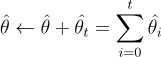
  along it (with a minus sign — after all, we want to decrease the error, not increase it). And that's it, we just need to somehow initialize our first approximation
  and choose how many iterations we'll continue this procedure for. In our memory-inefficient way of storing approximations , the naive algorithm will look as follows:

 repeat:
at the current approximation
repeat:
at the current approximation 
 based on the calculated gradient
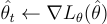 :
:

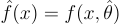 for its intended purpose
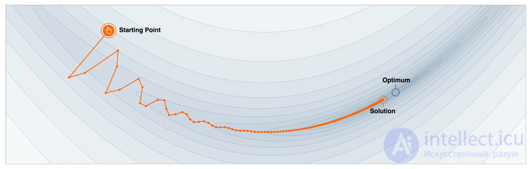
Let's expand our minds: imagine for a second that we can perform optimization in a functional space and iteratively look for approximations in the form of the functions themselves. Let's write out our approximation as a sum of incremental improvements, each of which is a function. For convenience, we'll immediately count this sum starting from the initial approximation  :
:
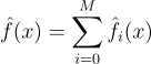
No magic has happened yet, we've simply decided that we'll look for our approximation not in the form of one big model with a bunch of parameters (like, for example, a neural network), but in the form of a sum of functions, pretending that this way we're moving through a functional space.
To solve the problem, we'll still have to restrict our search to some family of functions 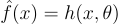 . But, first, a sum of models can be more complex than any single model from this family (a sum of two depth-1 stump trees can no longer be approximated by a single stump). Second, the overall problem is still happening in a functional space. Let's immediately take into account that at each step, for the functions, we'll need to pick an optimal coefficient
  . For step
  the problem looks as follows:

And now it's time for the magic. We wrote out all our problems in general form, as if we could just go ahead and train any models  whatsoever with respect to any loss functions
  whatsoever. In practice, this is extremely difficult, so a simple way was devised to reduce the problem to something solvable.
Knowing the expression for the gradient of the loss function, we can calculate its values on our data. So let's train the models so that our predictions are most correlated with this gradient (with a minus sign). That is, we'll be solving an OLS regression problem, trying to fit predictions to these residuals. For classification, for regression, and for ranking, under the hood we'll always be minimizing the squared difference between the pseudo-residuals  and our predictions. For step the final problem looks as follows:


Now we have everything we need to finally write out the GBM algorithm proposed by Jerome Friedman in 1999. We're still solving the general supervised learning problem. To run the algorithm, we need to gather several components:
;; with its gradient written out;, with a training procedure for them;, for example, the tree depth for decision trees;
The only point that's been left unattended — the initial approximation  . For simplicity, a simple constant value
  is used as the initialization. It, as well as the optimal coefficient
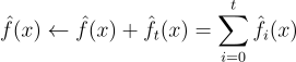
  , is found by binary search, or another line search algorithm, with respect to the original loss function (not the gradient). So, the GBM algorithm:

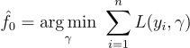 repeat:


 as a regression on the pseudo-residuals
 for with respect to the original loss function

Let's try to figure out how GBM works using a toy example. We'll use it to recover a noisy function  .
.
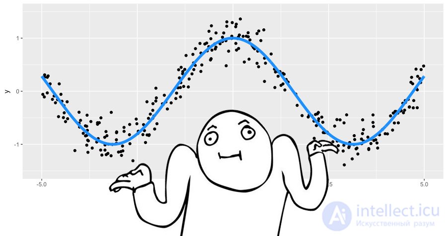
This is a regression problem on a real-valued target variable, so we'll use the mean squared error loss function. We'll generate 300 pairs of observations, and we'll approximate with decision trees of depth 2. Let's put together everything we need to apply GBM:
 ✓
✓ ✓;
✓; ✓
✓ of the loss is simply the residuals
  ✓;
✓; ✓;
✓;
For the mean squared error, everything is simple, both for the initialization and for the coefficients . Namely, we'll initialize GBM with the mean value 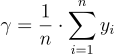 , and all equal 1.
Let's run GBM and plot two types of charts: the actual approximation (blue chart), and each tree we build  on its pseudo-residuals (green chart). The chart number corresponds to the iteration number:
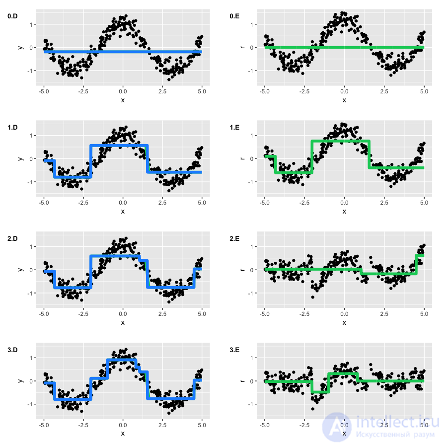
Notice that by the second iteration our trees had reproduced the main shape of the function. However, at the first iteration we can see that the algorithm only built the "left branch" of the function ( ). This simply happened because our trees didn't have enough depth to build the symmetric branch right away, and the error on the left branch was larger. So the right branch "grew in" only at the second iteration.
Otherwise, the process went exactly as we expected: at each step our pseudo-residuals decreased, and GBM approximated the original cosine more and more closely. However, trees, by their construction, cannot approximate a continuous function, so in this example GBM is useful but not perfect. To play around with how GBM approximates functions yourself, the Brilliantly wrong blog has an awesome interactive demo:
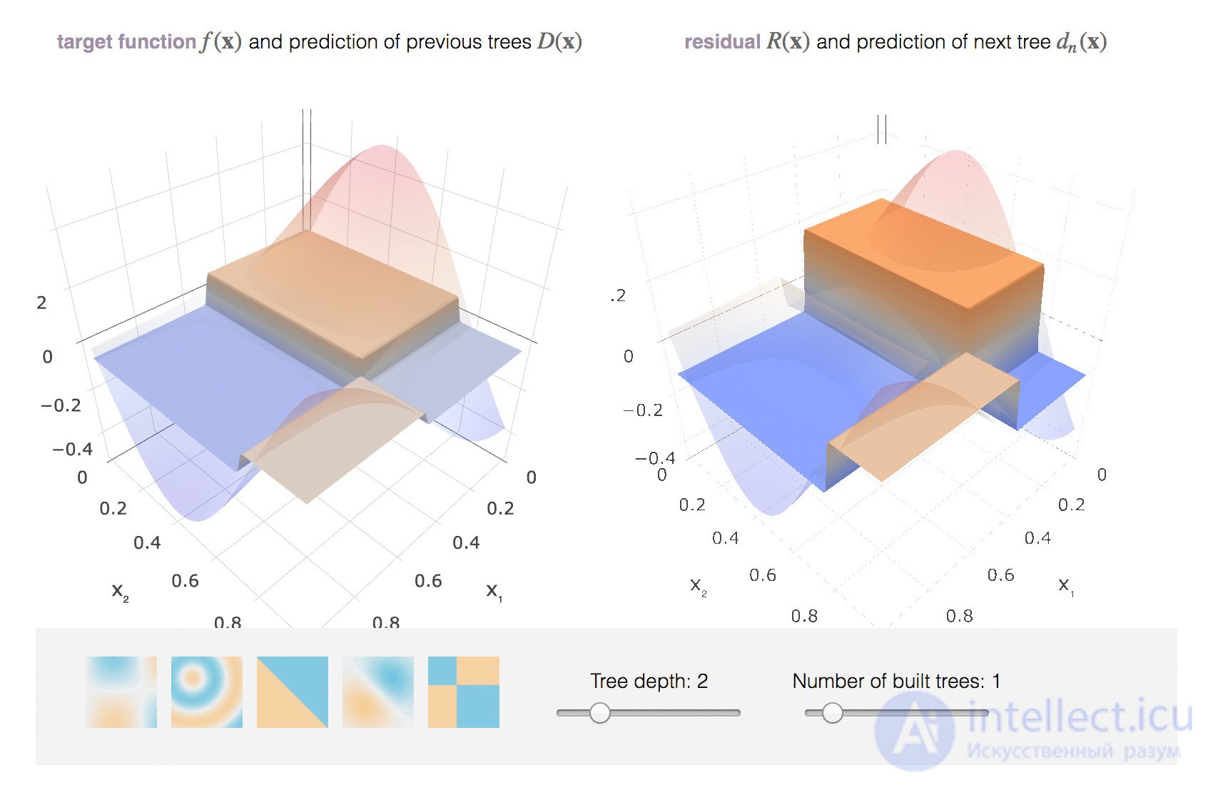
http://arogozhnikov.github.io/2016/06/24/gradient_boosting_explained.html
What should we do if we want to solve not ordinary mean-squared regression, but, say, a binary classification task? No problem — we just need to choose, for the target variable , a loss function appropriate to the task. This is the most important high-level decision, which determines exactly what we will be optimizing and what properties to expect from our final model.
As a rule, we don't need to come up with or derive anything ourselves — researchers have already done it all for us. Today we'll go through the loss functions for the two most commonly encountered tasks: regression  and binary classification
  . What to do about multiclass classification, ranking, and various intermediate cases like integer regression, we'll cover another time.
Let's start with regression . When choosing a loss function in this case, we are first of all deciding exactly which property of the conditional distribution  we want to recover. The most common options are:
, also known as  loss, also known as Gaussian loss. This is the classic conditional mean, the most common and simplest option. If there is no additional information or robustness requirements for the model — use this one.
 , also known as
  loss, also known as Laplacian loss. This, at first glance, not-very-differentiable thing, actually defines the conditional median. The median, as we know, is more robust to outliers, so in some tasks this loss function is preferable, since it penalizes large deviations much less harshly than the quadratic function.
 loss, also known as Quantile loss. If, say, we wanted not the conditional median with , but the conditional 75% quantile, we would use this variant with
  . You can see that this function is asymmetric and penalizes observations on the side of the quantile we need more heavily.
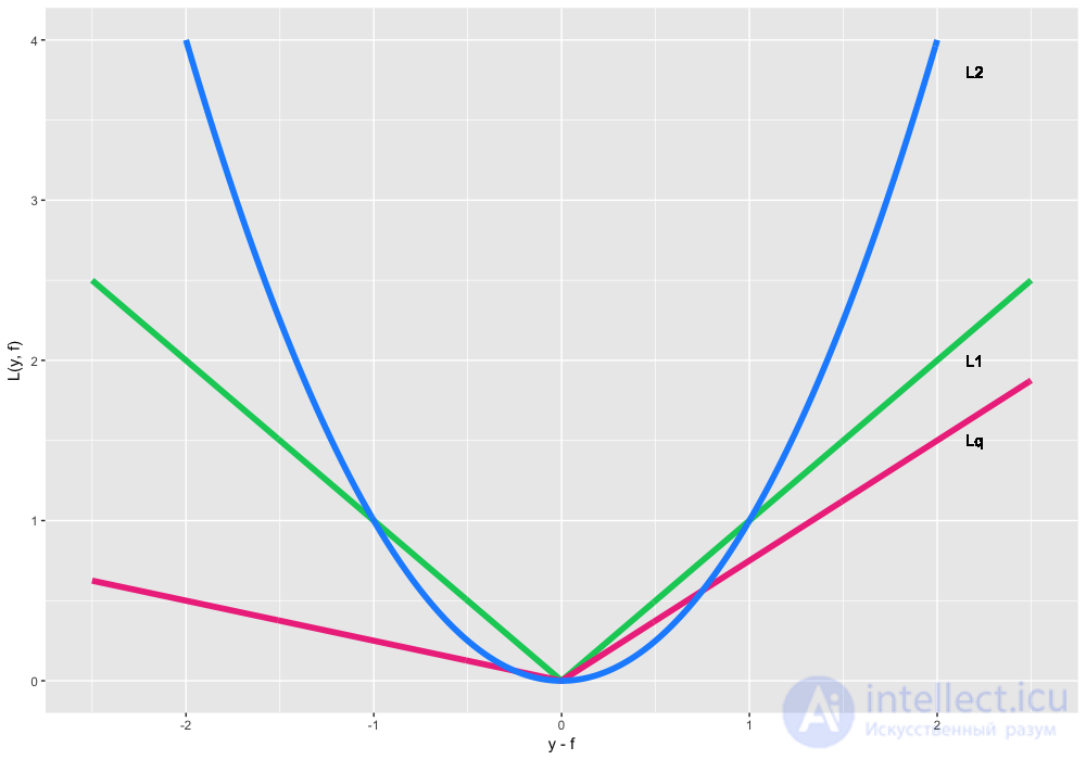
Let's try using the loss function on our toy data, trying to recover the conditional 75% quantile of the cosine. Let's put it all together:
✓ ✓; — an indicator function, weighted by our . We will be training trees on something very similar to a classifier:
 ✓; ✓;
✓; ✓;
We have an obvious initial approximation — simply take the quantile we need . However, we know nothing about the optimal coefficients , so we'll use a standard line search. Let's see what we got:
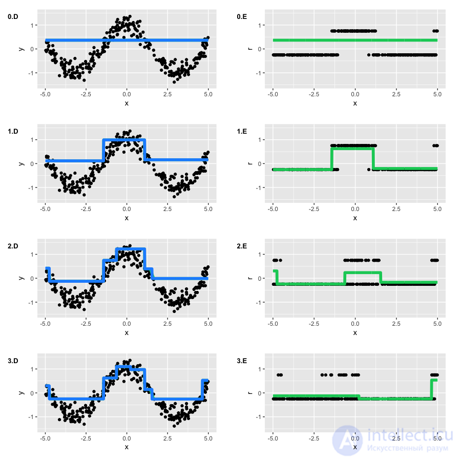
It's unusual to see that in fact we are training on something very unlike ordinary residuals — at each iteration  take only two possible values. However, the result of GBM's work is quite similar to our original function.
If we let the algorithm keep training on this toy example, we get almost the same result as with the quadratic loss function, shifted by  . But if we were looking for quantiles above 90%, computational difficulties could arise. Namely, if the ratio of the number of points above the desired quantile is too small (like imbalanced classes), the model won't be able to train well. It's worth thinking about such nuances when solving atypical tasks.
A bit more about regression loss functions
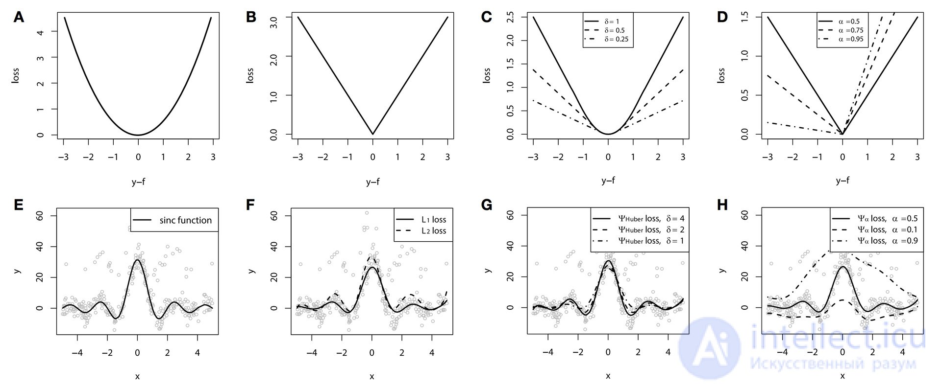
Quite a lot of loss functions have been developed for the regression task, including ones with additional robustness properties. One such example is the Huber loss function. The essence of this function is that for small deviations it behaves like , and starting from a preset threshold, it starts behaving like . This makes it possible to reduce the contribution of outliers and the quadratically large errors that follow from them on the overall shape of the function, without focusing too much attention on small inaccuracies and deviations.
We can look at how this loss function works on the following toy example. As a base we'll take toy data for the function  , to which special noise has been added: a mixture of a Gaussian distribution and a Bernoulli distribution, acting as a one-sided outlier generator. The loss functions themselves are shown in charts A-D, and the corresponding GBMs are shown in charts F-H (chart E shows the original function):
And in high resolution.
In this example, splines were used as the base algorithms for visual clarity. After all, we already mentioned that you can boost more than just trees, right?
Based on the results of the example, due to the artificially created noise problem, the difference between , and Huber loss is quite noticeable. With a well-chosen Huber loss parameter, we can even get the best approximation of the function among our options. This example also clearly shows the difference in the conditional quantiles (10%, 50%, and 90% in our case).
Unfortunately, the Huber loss function is not implemented in all modern libraries (it's implemented in h2o, but not yet in xgboost). The same applies to other interesting loss functions, including conditional quantiles and such exotic things as conditional expectiles. But in general, it's quite useful to know that such options exist and can be used.
Now let's look at binary classification, where . We've already seen that GBM can be used to optimize even not-very-differentiable loss functions. In fact, one could, without thinking too much, try to solve this case as just another regression task with some loss, but that wouldn't be quite right (although it's possible).
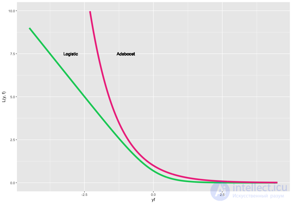
Because of the fundamentally different nature of the target variable's distribution, we will predict and optimize not the class labels themselves, but their log-likelihood. To do this, we reformulate the loss functions over the product of the predictions and the true labels  (it's no accident that we chose labels of different signs). The best-known variants of such classification loss functions are:
 , also known as Logistic loss, also known as Bernoulli loss. An interesting property is that we penalize even correctly predicted class labels. No, that's not a bug. On the contrary, by optimizing this loss function we can keep "pushing apart" the classes and improving the classifier even when all observations are predicted correctly. This is the most standard and frequently used loss function in binary classification.
 , also known as Adaboost loss. As it turns out, the classic Adaboost algorithm is equivalent to GBM with this loss function. Conceptually, this loss function is very similar to Logistic loss, but has a harsher exponential penalty for classification errors and is used less often.
Let's generate new toy data for the classification task. As a base, we'll take our noisy cosine, and use the sign function for the target variable's classes. The new data looks as follows (jitter noise has been added for clarity):
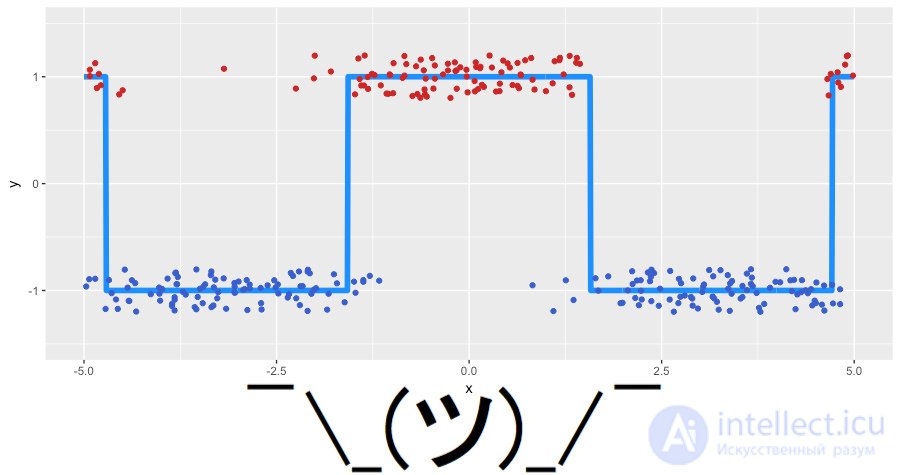
Let's use Logistic loss to see what we're actually boosting. As before, let's put together what we'll be solving:
 ✓ ✓;
✓ ✓; ✓; ✓;
✓; ✓;
This time the algorithm's initialization is a bit more complicated. First, our classes are imbalanced and split roughly 63% to 37%. Second, no analytical formula for initialization is known for our loss function. So we'll search for  using a search:
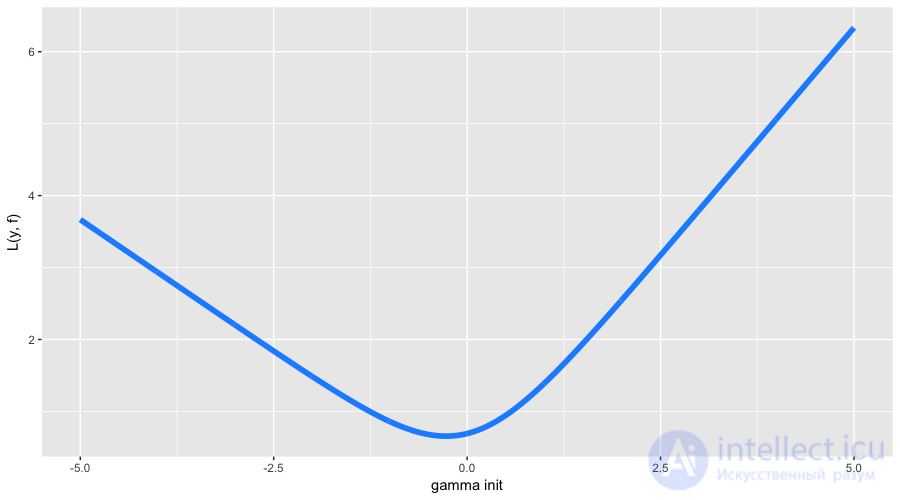
The optimal initial approximation was found to be around -0.273. One could have guessed that it would be negative (it's more advantageous for us to predict everyone as the most popular class), but as we already said, there's no formula for the exact value. Now let's finally run GBM and see what's actually happening under the hood:
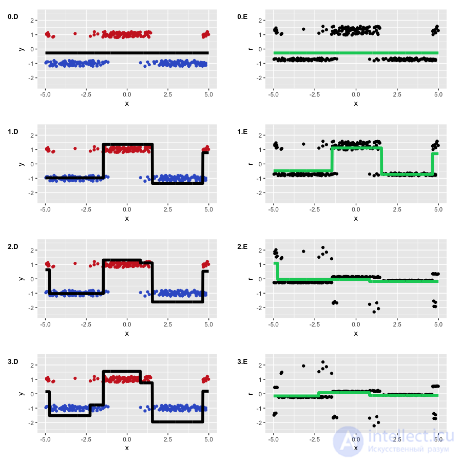
The algorithm worked successfully, recovering the separation of our classes. You can see how the "lower" regions are separated, where the trees are more confident about correctly predicting the negative class, and how two steps form, where the classes were mixed. In the pseudo-residuals, you can see that we have quite a lot of correctly classified observations, and some number of observations with large errors that appeared due to noise in the data. This is roughly what GBM is actually predicting in the classification task (regression on the pseudo-residuals of the logistic loss function).
Sometimes a situation arises where we want to come up with a more task-specific loss function. For example, when predicting financial time series we might want to give more weight to large movements of the time series, and in the customer churn prediction task — we'd rather better predict churn for customers with a high LTV (lifetime value, how much money a customer will bring us in the future).
The true path of the statistical warrior — come up with your own loss function, derive its derivative (and, for more efficient training, its Hessian too), and carefully check whether this function satisfies the required properties. However, there's a high chance of making a mistake somewhere, running into computational difficulties, and overall spending an unreasonable amount of time on research.
Instead, a very simple tool was invented that is rarely remembered in practice — weighting observations and defining weight functions. The simplest example of such weighting is setting weights to balance classes. In the general case, if we know that some subset of the data, whether in the input variables or in the target variable , has greater importance for our model, we simply assign it a larger weight  . The main thing is to satisfy the general reasonableness requirements for the weights:

Weights make it possible to significantly cut down the time spent adapting the loss function itself to the task at hand, and also encourage experimentation with the target properties of models. Exactly how to set these weights is purely our own creative task. From the point of view of the GBM algorithm and the optimization, we simply add scalar weights, turning a blind eye to their nature:

It's clear that for arbitrary weights we don't know any nice statistical properties of our model. In general, by tying the weights to the values , we can shoot ourselves in the foot. For example, using weights proportional to  in the loss function is not equivalent to loss, since the gradient won't take into account the values of the predictions themselves .
We're discussing all this to better understand our capabilities. Let's come up with some very exotic example of weights on our toy data. Let's define a strongly asymmetric weight function as follows:
$$display$$ \large \begin{equation} w(x) =\left\{ \begin{array}{@{}ll@{}} 0.1, & \text{if}\ x \leq 0 \\ 0.1 + |cos(x)|, & \text{if}\ x >0 \end{array}\right. \end{equation} $$display$$
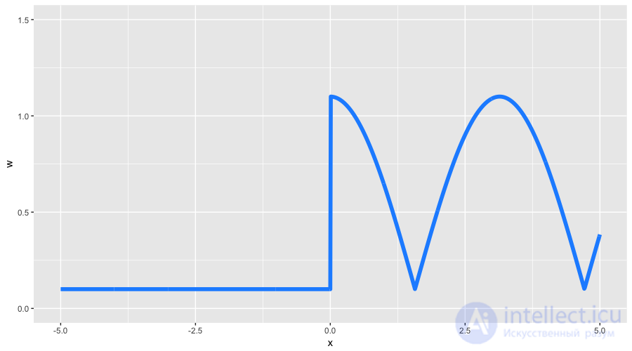
With these weights we expect to see two properties: less detail at negative values , and a function shape that more closely resembles the original cosine. We take all other GBM settings from our previous classification example, including the line search for the optimal coefficients. Let's see what we got:
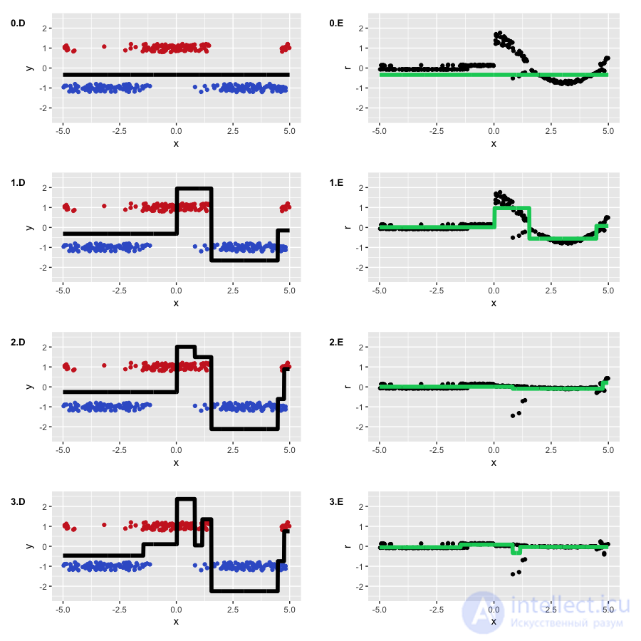
The result turned out just as we expected. First, we can see how much our pseudo-residuals started to differ, largely repeating our original cosine at the initial iteration. Second, the left part of the function's graph was largely ignored in favor of the right part, which had larger weights. Third, the function we obtained at the third iteration gained quite a lot of detail, becoming more similar to the original cosine (while also starting to slightly overfit).
Weights are a powerful tool that, at our own risk, allow us to significantly control the properties of our model. If you want to optimize your own loss function, it's worth first trying to solve a simpler task, but adding observation weights to it as you see fit.
Today we went through the main theory of gradient boosting. GBM is not just some specific algorithm, but a general methodology for building ensembles of models. Moreover, the methodology is quite flexible and extensible: you can train a large number of models taking into account various loss functions, while also hanging various kinds of weight functions on them.
As both practice and experience from machine learning competitions show, in standard tasks (everything except images and audio, as well as heavily sparse data), GBM is very often the most effective algorithm (not counting stacking and top-level ensembles, where GBM is almost always an integral part of them). There are also adaptations of GBM for Reinforcement Learning (Minecraft, ICML 2016), and the Viola-Jones algorithm, still used in computer vision today, is based on Adaboost.
In this article, we deliberately left out the questions related to GBM regularization, stochasticity, and the algorithm hyperparameters associated with them. It is not by chance that we chose a small number of algorithm iterations everywhere, . If we had chosen not 3 but 30 trees and run GBM as described above, the result would have turned out less predictable:
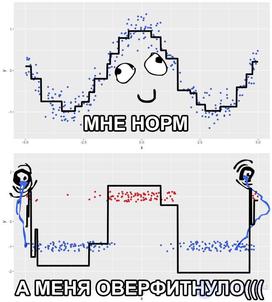
We will tell you about what to do in such situations, and how the GBM regularization parameters are related to each other, as well as the hyperparameters of the base algorithms, in the next article. In it we will also cover modern packages — xgboost, lightgbm and h2o, and practice tuning them correctly. In the meantime, we suggest you play around with the GBM settings in yet another very cool interactive demo, Brliiantly wrong:
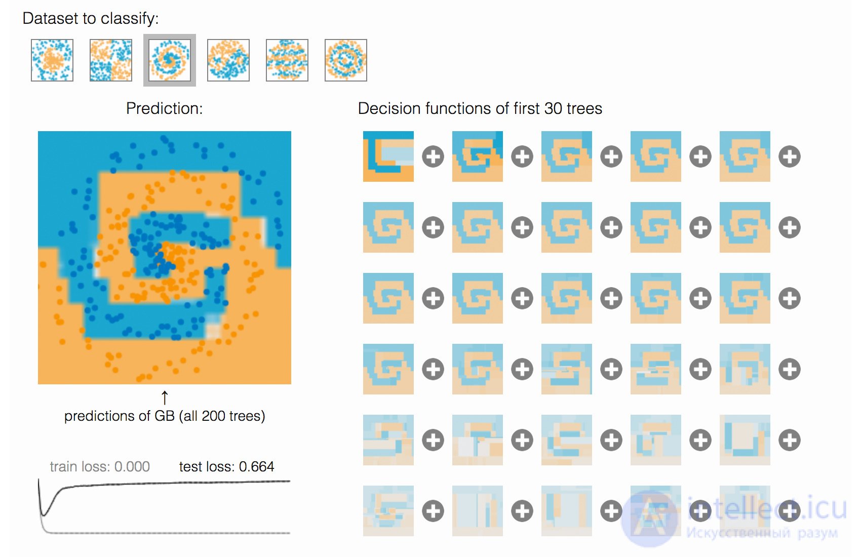
http://arogozhnikov.github.io/2016/07/05/gradient_boosting_playground.html
Current homework assignments are announced during the next session of the course; you can follow them in the VK group and in the course repository.
As an exercise, complete this assignment — you need to beat a simple baseline in the Kaggle Inclass competition on predicting flight delays.

Comments