4. Where logistic regression is good and where it is

Это окончание невероятной информации про линейные модели классификации.

...

Linear Models for Classification and Regression" > and train a logistic regression with regularization parameter . Let's plot the separating boundary.
Let's also check the classifier's accuracy on the training set. We see that the regularization turned out to be too strong, and the model is "underfitted". The classifier's accuracy on the training set turned out to be 0.627.

Code

poly = PolynomialFeatures(degree=7)
X_poly = poly.fit_transform(X)

C = 1e-2
logit = LogisticRegression(C=C, n_jobs=-1, random_state=17)
logit.fit(X_poly, y)

plot_boundary(logit, X, y, grid_step=.01, poly_featurizer=poly)

plt.scatter(X[y == 1, 0], X[y == 1, 1], c='green', label='Passed')
plt.scatter(X[y == 0, 0], X[y == 0, 1], c='red', label='Defective')
plt.xlabel("Test 1")
plt.ylabel("Test 2")
plt.title('2 microchip tests. Logit with C=0.01')
plt.legend();

print("Classifier accuracy on the training set:",
round(logit.score(X_poly, y), 3))

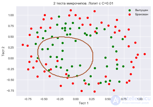
Let's increase to 1. By doing this, we weaken the regularization, so now the logistic regression weight values can turn out to be larger (in absolute value) than in the previous case. Now the classifier's accuracy on the training set is 0.831.

Code

C = 1
logit = LogisticRegression(C=C, n_jobs=-1, random_state=17)
logit.fit(X_poly, y)

plot_boundary(logit, X, y, grid_step=.005, poly_featurizer=poly)

plt.scatter(X[y == 1, 0], X[y == 1, 1], c='green', label='Passed')
plt.scatter(X[y == 0, 0], X[y == 0, 1], c='red', label='Defective')
plt.xlabel("Test 1")
plt.ylabel("Test 2")
plt.title('2 microchip tests. Logit with C=1')
plt.legend();

print("Classifier accuracy on the training set:",
round(logit.score(X_poly, y), 3))

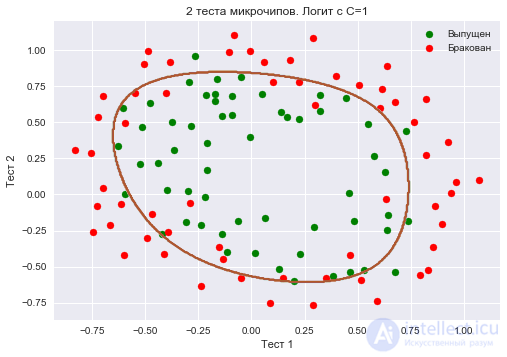
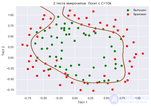
Let's increase even further – to 10 thousand. Now the regularization is clearly insufficient, and we observe overfitting. Note that in the previous case (with =1 and a "smooth" boundary), the model's accuracy on the training set is not much lower than in the 3rd case, but on new data, one can imagine that model 2 will perform much better.
The classifier's accuracy on the training set is 0.873.

Code

C = 1e4
logit = LogisticRegression(C=C, n_jobs=-1, random_state=17)
logit.fit(X_poly, y)

plot_boundary(logit, X, y, grid_step=.005, poly_featurizer=poly)

plt.scatter(X[y == 1, 0], X[y == 1, 1], c='green', label='Passed')
plt.scatter(X[y == 0, 0], X[y == 0, 1], c='red', label='Defective')
plt.xlabel("Test 1")
plt.ylabel("Test 2")
plt.title('2 microchip tests. Logit with C=10k')
plt.legend();

print("Classifier accuracy on the training set:",
round(logit.score(X_poly, y), 3))

To discuss the results, let's rewrite the formula for the functional optimized in logistic regression in the following form:

where

• – the logistic loss function, summed over the whole training set
• – the inverse regularization coefficient (the very same in the sklearn implementation of LogisticRegression)

Intermediate conclusions:

• the larger the parameter , the more complex the dependencies in the data the model can recover (intuitively, corresponds to the "complexity" of the model (model capacity))
• if the regularization is too strong (small values of ), the solution of the logistic loss minimization problem may end up with many weights vanishing or becoming too small. It is also said that the model is not "penalized" enough for errors (that is, in the functional the sum of squared weights "outweighs" the error , which can be relatively large). In such a case the model turns out to be underfitted (case 1)
• conversely, if the regularization is too weak (large values of ), the solution of the optimization problem can be a vector with large components in absolute value. In such a case the greater contribution to the optimized functional comes from and, loosely speaking, the model is too "afraid" of making mistakes on the training set objects, so it turns out to be overfitted (case 3)
• logistic regression itself will not "understand" (or, as is also said, will not "learn") which value of to choose, that is, this cannot be determined by solving the optimization problem that logistic regression represents (unlike the weights ). In exactly the same way, a decision tree cannot "figure out by itself" which depth limit to choose (within a single training process). That is why is a model hyperparameter that is tuned via cross-validation, just like max_depth for a tree.

Tuning the regularization parameter

Now let's find the optimal (in this example) value of the regularization parameter . This can be done using LogisticRegressionCV – a grid search over parameters followed by cross-validation. This class was created specifically for logistic regression (efficient parameter search algorithms are known for it); for an arbitrary model we would use GridSearchCV, RandomizedSearchCV, or, for example, special hyperparameter optimization algorithms implemented in hyperopt.

Code

skf = StratifiedKFold(n_splits=5, shuffle=True, random_state=17)

c_values = np.logspace(-2, 3, 500)

logit_searcher = LogisticRegressionCV(Cs=c_values, cv=skf, verbose=1, n_jobs=-1)
logit_searcher.fit(X_poly, y)

Let's see how the quality of the model (accuracy on the training and validation sets) changes as the hyperparameter changes.

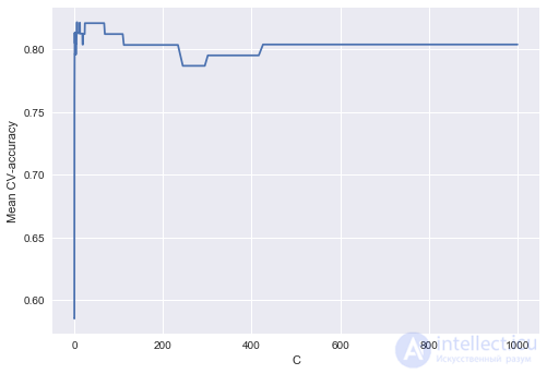
Let's highlight the region with the "best" values of C.

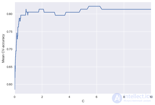
As we remember, such curves are called validation curves; earlier we plotted them by hand, but sklearn has special methods for building them, which we will now use as well.

4. Where logistic regression is good and where it is not so good

Analysis of IMDB movie reviews

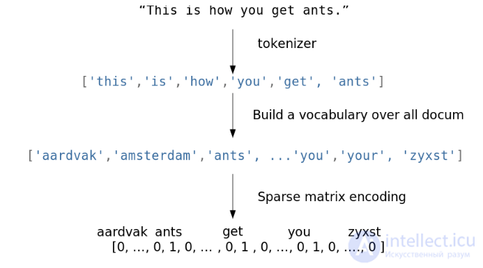
We will solve the binary classification problem for IMDB movie reviews. There is a training set with labeled reviews: 12500 reviews are known to be good, and another 12500 are known to be bad. Here it is no longer so simple to jump straight into machine learning, because there is no ready-made matrix – it needs to be prepared. We will use the simplest approach – the bag of words. In this approach, the features of a review are indicators of the presence in it of each word from the entire corpus, where the corpus is the set of all reviews. The idea is illustrated by the picture

Importing libraries and loading the data

from __future__ import division, print_function
# turn off various Anaconda warnings
import warnings
warnings.filterwarnings('ignore')
import numpy as np
import matplotlib.pyplot as plt
%matplotlib inline
import seaborn as sns
import numpy as np
from sklearn.datasets import load_files
from sklearn.feature_extraction.text import CountVectorizer, TfidfTransformer, TfidfVectorizer
from sklearn.linear_model import LogisticRegression
from sklearn.svm import LinearSVC

Let's load the data from here (a brief description — here). The training and test sets each have 12500 good and 12500 bad movie reviews.

reviews_train = load_files("YOUR PATH")
text_train, y_train = reviews_train.data, reviews_train.target

print("Number of documents in training data: %d" % len(text_train))
print(np.bincount(y_train))

# change the file path
reviews_test = load_files("YOUR PATH")
text_test, y_test = reviews_test.data, reviews_test.target
print("Number of documents in test data: %d" % len(text_test))
print(np.bincount(y_test))

An example of a bad review:

'Words can\'t describe how bad this movie is. I can\'t explain it by writing only. You have too see it for yourself to get at grip of how horrible a movie really can be. Not that I recommend you to do that. There are so many clich , mistakes (and all other negative things you can imagine) here that will just make you cry. To start with the technical first, there are a LOT of mistakes regarding the airplane. I won\'t list them here, but just mention the coloring of the plane. They didn\'t even manage to show an airliner in the colors of a fictional airline, but instead used a 7479 painted in the original Boeing livery. Very bad. The plot is stupid and has been done many times before, only much, much better. There are so many ridiculous moments here that i lost count of it really early. Also, I was on the bad guys\' side all the time in the movie, because the good guys were so stupid. "Executive Decision" should without a doubt be you\'re choice over this one, even the "Turbulence"-movies are better. In fact, every other movie in the world is better than this one.'

It's impossible to describe in words how bad this movie is. I can't explain it just by writing. You have to see it for yourself to understand how horrible a movie can really be. Not that I'm recommending you do that. There are so many clich s, mistakes (and every other negative thing you can imagine) here that it will just make you cry. Let's start with the technical issues. There are A LOT of mistakes regarding the airplane. I won't list them all here, but I'll just mention the plane's paint job. They didn't even manage to show an airliner in the colors of a fictional airline, and instead used a 7479 painted in the original Boeing livery. Very bad. The plot is stupid, and has been done many times before, only much, much better. There are so many ridiculous moments here that I lost count really early on. Also, I was on the bad guys' side the whole time in the movie, because the good guys were so stupid. "Executive Decision" should without a doubt be your pick over this one; even the "Turbulence" movies are better. In fact, every other movie in the world is better than this one ».

An example of a good review:

'Everyone plays their part pretty well in this "little nice movie". Belushi gets the chance to live part of his life differently, but ends up realizing that what he had was going to be just as good or maybe even better. The movie shows us that we ought to take advantage of the opportunities we have, not the ones we do not or cannot have. If U can get this movie on video for around $10, it\xc2\xb4d be an investment!'

«Everyone plays their part well in this« nice little movie ». Belushi gets a chance to live part of his life differently, but ends up realizing that what he had was going to be just as good, or maybe even better. The movie shows us that we should make use of the opportunities we have, not the ones we don't have or can't have. If you can get this movie on video for around $10, that would be money well invested! '

Simple word counting

Let's build a vocabulary of all the words using CountVectorizer. In total, the training set has 74849 unique words. If we look at examples of the resulting "words" (it's better to call them tokens), we can see that we have skipped many important text processing steps here (automatic text processing could be the topic of a separate series of articles).

Code

cv = CountVectorizer()
cv.fit(text_train)

print(len(cv.vocabulary_)) #74849

print(cv.get_feature_names()[:50])
print(cv.get_feature_names()[50000:50050])

['00', '000', '0000000000001', '00001', '00015', '000s', '001', '003830', '006', '007', '0079', '0080', '0083', '0093638', '00am', '00pm', '00s', '01', '01pm', '02', '020410', '029', '03', '04', '041', '05', '050', '06', '06th', '07', '08', '087', '089', '08th', '09', '0f', '0ne', '0r', '0s', '10', '100', '1000', '1000000', '10000000000000', '1000lb', '1000s', '1001', '100b', '100k', '100m']
['pincher', 'pinchers', 'pinches', 'pinching', 'pinchot', 'pinciotti', 'pine', 'pineal', 'pineapple', 'pineapples', 'pines', 'pinet', 'pinetrees', 'pineyro', 'pinfall', 'pinfold', 'ping', 'pingo', 'pinhead', 'pinheads', 'pinho', 'pining', 'pinjar', 'pink', 'pinkerton', 'pinkett', 'pinkie', 'pinkins', 'pinkish', 'pinko', 'pinks', 'pinku', 'pinkus', 'pinky', 'pinnacle', 'pinnacles', 'pinned', 'pinning', 'pinnings', 'pinnochio', 'pinnocioesque', 'pino', 'pinocchio', 'pinochet', 'pinochets', 'pinoy', 'pinpoint', 'pinpoints', 'pins', 'pinsent']

Let's encode the sentences from the training set texts with the indices of the words they contain. We will use a sparse format. We will transform the test set the same way.

X_train = cv.transform(text_train)
X_test = cv.transform(text_test)

Let's train a logistic regression and look at the accuracy on the training and test sets. It turns out that on the test set we correctly guess the sentiment of about 86.7% of the reviews.

Code

%%time
logit = LogisticRegression(n_jobs=-1, random_state=7)
logit.fit(X_train, y_train)
print(round(logit.score(X_train, y_train), 3), round(logit.score(X_test, y_test), 3))

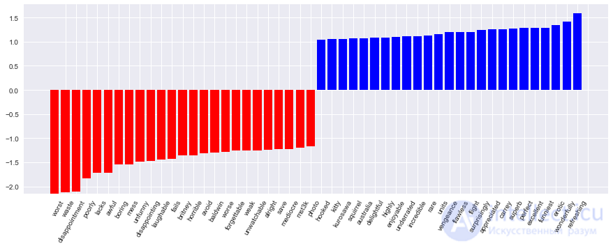
The model's coefficients can be visualized nicely.

Code for visualizing the model's coefficients

def visualize_coefficients(classifier, feature_names, n_top_features=25):
# get coefficients with large absolute values
coef = classifier.coef_.ravel()
positive_coefficients = np.argsort(coef)[-n_top_features:]
negative_coefficients = np.argsort(coef)[:n_top_features]
interesting_coefficients = np.hstack([negative_coefficients, positive_coefficients])
# plot them
plt.figure(figsize=(15, 5))
colors = ["red" if c < 0 else "blue" for c in coef[interesting_coefficients]]
plt.bar(np.arange(2 * n_top_features), coef[interesting_coefficients], color=colors)
feature_names = np.array(feature_names)
plt.xticks(np.arange(1, 1 + 2 * n_top_features), feature_names[interesting_coefficients], rotation=60, ha="right");

def plot_grid_scores(grid, param_name):
plt.plot(grid.param_grid[param_name], grid.cv_results_['mean_train_score'],
color='green', label='train')
plt.plot(grid.param_grid[param_name], grid.cv_results_['mean_test_score'],
color='red', label='test')
plt.legend();

visualize_coefficients(logit, cv.get_feature_names())

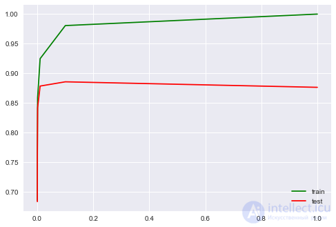
Let's tune the regularization coefficient for the logistic regression. We will use sklearn.pipeline, since CountVectorizer should only be applied correctly to the data on which the model is currently being trained (so as not to "peek" into the test set and not compute word occurrence frequencies from it). In this case, the pipeline specifies a sequence of actions: apply CountVectorizer, then train the logistic regression. This way we raise the accuracy to 88.5% on cross-validation and 87.9% on the held-out set.

Code

from sklearn.pipeline import make_pipeline

text_pipe_logit = make_pipeline(CountVectorizer(),
LogisticRegression(n_jobs=-1, random_state=7))

text_pipe_logit.fit(text_train, y_train)
print(text_pipe_logit.score(text_test, y_test))

from sklearn.model_selection import GridSearchCV

param_grid_logit = {'logisticregression__C': np.logspace(-5, 0, 6)}
grid_logit = GridSearchCV(text_pipe_logit, param_grid_logit, cv=3, n_jobs=-1)

grid_logit.fit(text_train, y_train)
grid_logit.best_params_, grid_logit.best_score_
plot_grid_scores(grid_logit, 'logisticregression__C')
grid_logit.score(text_test, y_test)

Now the same thing, but with a random forest. We see that with logistic regression we achieve a higher accuracy with less effort. The forest takes longer to run, and on the held-out set gives 85.5% accuracy.

Code for training a random forest

from sklearn.ensemble import RandomForestClassifier
forest = RandomForestClassifier(n_estimators=200, n_jobs=-1, random_state=17)
forest.fit(X_train, y_train)
print(round(forest.score(X_test, y_test), 3))

The XOR problem

Now let's look at an example where linear models perform worse.

Linear classification methods construct a very simple separating surface after all – a hyperplane. The most famous toy example in which the classes cannot be split by a hyperplane (that is, by a straight line, if it's 2D) without errors, got the name "the XOR problem".

XOR is "exclusive OR", a boolean function with the following truth table:

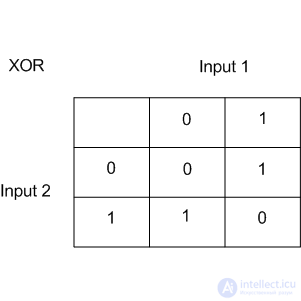
XOR gave its name to a simple binary classification problem, in which the classes are represented by intersecting clouds of points stretched along the diagonals.

Code that draws the following 3 pictures

# generate the data
rng = np.random.RandomState(0)
X = rng.randn(200, 2)
y = np.logical_xor(X[:, 0] > 0, X[:, 1] > 0)

plt.scatter(X[:, 0], X[:, 1], s=30, c=y, cmap=plt.cm.Paired);

def plot_boundary(clf, X, y, plot_title):
xx, yy = np.meshgrid(np.linspace(-3, 3, 50),
np.linspace(-3, 3, 50))
clf.fit(X, y)
# plot the decision function for each datapoint on the grid
Z = clf.predict_proba(np.vstack((xx.ravel(), yy.ravel())).T)[:, 1]
Z = Z.reshape(xx.shape)

image = plt.imshow(Z, interpolation='nearest',
extent=(xx.min(), xx.max(), yy.min(), yy.max()),
aspect='auto', origin='lower', cmap=plt.cm.PuOr_r)
contours = plt.contour(xx, yy, Z, levels= , linewidths=2,
linetypes='--')
plt.scatter(X[:, 0], X[:, 1], s=30, c=y, cmap=plt.cm.Paired)
plt.xticks(())
plt.yticks(())
plt.xlabel(r'$$')
plt.ylabel(r'$$')
plt.axis([-3, 3, -3, 3])
plt.colorbar(image)
plt.title(plot_title, fontsize=12);

plot_boundary(LogisticRegression(), X, y,
"Logistic Regression, XOR problem")

from sklearn.preprocessing import PolynomialFeatures
from sklearn.pipeline import Pipeline

logit_pipe = Pipeline([('poly', PolynomialFeatures(degree=2)),
('logit', LogisticRegression())])

plot_boundary(logit_pipe, X, y,
"Logistic Regression + quadratic features. XOR problem")

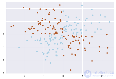
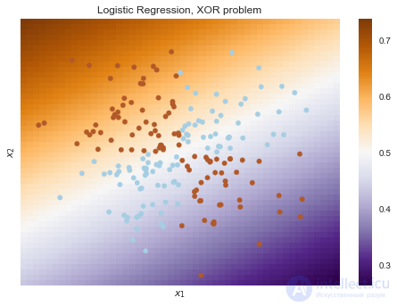
Obviously, you cannot draw a straight line in such a way as to separate one class from the other without errors. That is why logistic regression handles this task poorly.

But if we feed in polynomial features, in this case up to degree 2, then the problem is solved.

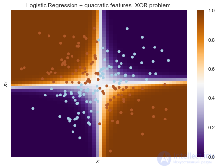
Here logistic regression still constructed a hyperplane, but in a 6-dimensional feature space and . In the projection onto the original feature space the boundary turned out to be nonlinear.

In practice, polynomial features really do help, but constructing them explicitly is computationally inefficient. SVM with the kernel trick works much faster. In this approach, in a high-dimensional space only the distance between objects is computed (given by a kernel function), and there is no need to explicitly generate a combinatorially large number of features. You can read about this in detail in Evgeny Sokolov's course (the math there is already quite serious).

5. Validation and learning curves

We already have an idea of model validation, cross-validation, and regularization.
Now let's consider the main question:

If we are not satisfied with the quality of the model, what should we do?

• Make the model more complex or simplify it?
• Add more features?
• Or do we simply need more training data?

The answers to these questions are not always obvious. In particular, sometimes using a more complex model will lead to worse metrics. Or adding observations will not lead to any noticeable changes. The ability to make the right decision and choose the right way to improve the model is, in fact, what distinguishes a good specialist from a bad one.

We will work with the familiar data on customer churn of a telecom operator.

Importing libraries and reading the data

from __future__ import division, print_function
# turn off various Anaconda warnings
import warnings
warnings.filterwarnings('ignore')
%matplotlib inline
from matplotlib import pyplot as plt
import seaborn as sns

import numpy as np
import pandas as pd
from sklearn.preprocessing import PolynomialFeatures
from sklearn.pipeline import Pipeline
from sklearn.preprocessing import StandardScaler
from sklearn.linear_model import LogisticRegression, LogisticRegressionCV, SGDClassifier
from sklearn.model_selection import validation_curve

data = pd.read_csv('../../data/telecom_churn.csv').drop('State', axis=1)
data['International plan'] = data['International plan'].map({'Yes': 1, 'No': 0})
data['Voice mail plan'] = data['Voice mail plan'].map({'Yes': 1, 'No': 0})

y = data['Churn'].astype('int').values
X = data.drop('Churn', axis=1).values

We will train the logistic regression using stochastic gradient descent. For now let's just say it's because it's faster, but later in the course we have a separate article about this topic. Let's plot validation curves showing how the quality (ROC AUC) on the training and validation sets changes as the regularization parameter changes.

Code

alphas = np.logspace(-2, 0, 20)
sgd_logit = SGDClassifier(loss='log', n_jobs=-1, random_state=17)
logit_pipe = Pipeline([('scaler', StandardScaler()), ('poly', PolynomialFeatures(degree=2)),
('sgd_logit', sgd_logit)])
val_train, val_test = validation_curve(logit_pipe, X, y,
'sgd_logit__alpha', alphas, cv=5,
scoring='roc_auc')

def plot_with_err(x, data, **kwargs):
mu, std = data.mean(1), data.std(1)
lines = plt.plot(x, mu, '-', **kwargs)
plt.fill_between(x, mu - std, mu + std, edgecolor='none',
facecolor=lines .get_color(), alpha=0.2)

plot_with_err(alphas, val_train, label='training scores')
plot_with_err(alphas, val_test, label='validation scores')
plt.xlabel(r'$\alpha$'); plt.ylabel('ROC AUC')
plt.legend();

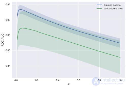
The trend is visible right away, and it is a very common one.

• For simple models, the training and validation error are close to each other, and both are large. This suggests that the model is underfitted: that is, it does not have enough parameters.

• For strongly overcomplicated models, the training and validation errors differ significantly. This can be explained by overfitting: when there are too many parameters or not enough regularization, the algorithm can get "distracted" by noise in the data and miss the main trend.

How much data do we need?

It is well known that the more data a model uses, the better. But how can we tell, in a specific situation, whether new data will help? Say, does it make sense for us to spend N\$ on the labor of assessors in order to double the sample size?

Since there may not be any new data available yet, it makes sense to vary the size of the existing training set and see how the quality of the solution depends on the amount of data the model was trained on. This is how learning curves are obtained.

The idea is simple: we plot the error as a function of the number of examples used for training. The model's parameters are fixed in advance.

Let's see what we get for a linear model. We will set the regularization coefficient to a large value.

Code

from sklearn.model_selection import learning_curve

def plot_learning_curve(degree=2, alpha=0.01):
train_sizes = np.linspace(0.05, 1, 20)
logit_pipe = Pipeline([('scaler', StandardScaler()), ('poly', PolynomialFeatures(degree=degree)),
('sgd_logit', SGDClassifier(n_jobs=-1, random_state=17, alpha=alpha))])
N_train, val_train, val_test = learning_curve(logit_pipe,
X, y, train_sizes=train_sizes, cv=5,
scoring='roc_auc')
plot_with_err(N_train, val_train, label='training scores')
plot_with_err(N_train, val_test, label='validation scores')
plt.xlabel('Training Set Size'); plt.ylabel('AUC')
plt.legend()

plot_learning_curve(degree=2, alpha=10)

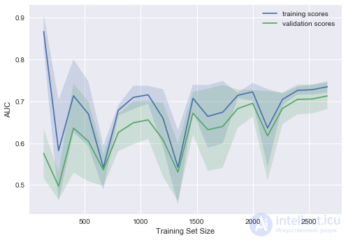
A typical situation: for a small amount of data, the errors on the training set and during cross-validation differ quite a lot, which indicates overfitting. For the same model but with a larger amount of data, the errors "converge", which indicates underfitting.

If we add more data, the error on the training set will not grow, but on the other hand, the error on the test data will not decrease either.

It turns out that the errors have "converged", and adding new data will not help. Actually, this case is the most interesting one for a business. There may be a situation where we increase the sample size 10-fold. But if we don't change the complexity of the model, this may not help at all. That is, the strategy of "tune it once, then reuse it 10 times" may not work.

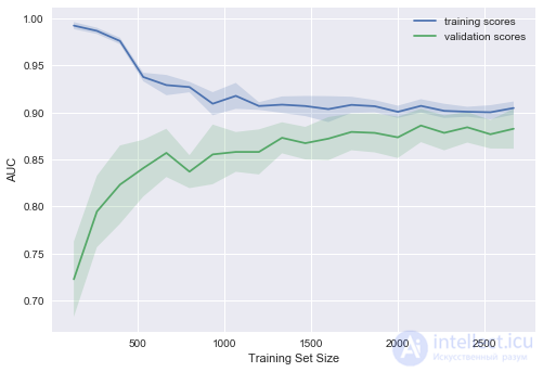
What happens if we change the regularization coefficient (decrease it to 0.05)?

We see a good trend – the curves gradually converge, and if we keep moving to the right (adding data to the model), we can further improve the quality on validation.

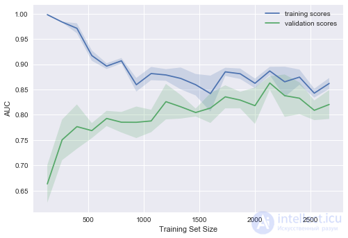
And what if we make the model even more complex ()?

Overfitting shows up – the AUC drops both on training and on validation.

By plotting curves like these, you can understand which direction to move in and how to properly tune the model's complexity on new data.

Conclusions on validation and learning curves

• The error on the training set by itself says nothing about the quality of the model
• The cross-validation error shows how well the model adapts to the data (the existing trend in the data), while retaining the ability to generalize to new data
• A validation curve is a graph showing the result on the training and validation sets as a function of the model's complexity:
• if the two curves are located close together, and both errors are large, — this is a sign of underfitting
• if the two curves are far apart from each other, — this is an indicator of overfitting
• A learning curve is a graph showing the results on validation and on the training subsample as a function of the number of observations:
• if the curves have converged to each other, adding new data will not help – you need to change the complexity of the model
• if the curves have not yet converged, adding new data may improve the result.

6. Advantages and disadvantages of linear models in machine learning problems

Pros:

• Well studied
• Very fast, can work on very large datasets
• Practically unmatched when there are a very large number of features (from hundreds of thousands and more), and they are sparse (although there are also factorization machines)
• The coefficients for the features can be interpreted (provided the features are scaled) – in linear regression as partial derivatives of the dependent variable with respect to the features, in logistic regression as the change in the odds of being assigned to one of the classes by a factor of when the feature changes by 1 unit, more details here
• Logistic regression produces probabilities of belonging to different classes (this is highly valued, for example, in credit scoring)
• The model can also construct a nonlinear boundary if polynomial features are fed as input

Cons:

• They perform poorly on problems where the dependence of the responses on the features is complex and nonlinear
• In practice, the assumptions of the Gauss-Markov theorem are almost never satisfied, so linear methods more often perform worse than, for example, SVM and ensembles (in terms of the quality of the classification/regression solution)

7. Independent work

Current homework assignments are announced during the next session of the course; you can follow them in the VK group and in the course repository.

To reinforce the material covered, we suggest the following assignment: figure out how TfidfVectorizer and DictVectorizer work, train and tune a Ridge linear regression model on data about publications on Habrahabr, and reproduce the benchmark in the competition. You can check yourself by submitting your answers via the web form (you will also find the solution there).

See also

• Regression
• Hardy–Weinberg principle
• Internal validity
• Law of large numbers
• Martingale
• Regression dilution
• Selection criterion
• Least squares method

Продолжение:

Часть 1 4. Linear Models for Classification and Regression
Часть 2 4. Where logistic regression is good and where it is