
Lecture
The fifth article of the course will focus on simple composition methods: bagging and random forest. You will learn how to obtain the distribution of the mean over a general population if we only have information about a small part of it; we will see how composing algorithms reduces variance and thus improves model accuracy; we will figure out what a random forest is, which of its parameters need to be «tuned», and how to find the most important feature. We will focus on practice, adding a «pinch» of math.
UPD: the course is now available in English under the mlcourse.ai brand, with articles on Medium and materials on Kaggle (Dataset) and on GitHub.
A video recording of the lecture based on this article, from the second run of the open course (September-November 2017).
List of articles in the series
Outline of this article
From previous lectures you have already learned about various classification algorithms, and you have learned how to validate correctly and evaluate model quality. But what should you do if you have already found the best model and can no longer improve its accuracy? In that case, you need to apply more advanced machine learning techniques, which can be grouped under the word «ensembles». An ensemble is a certain collection whose parts form a single whole. From everyday life you know musical ensembles, where several musical instruments are combined, architectural ensembles with different buildings, and so on.
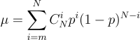
A good example of ensembles is considered to be Condorcet's jury theorem (1784). If each member of a jury has an independent opinion, and if the probability of a correct decision by a jury member is greater than 0.5, then the probability of a correct decision by the jury as a whole increases as the number of jury members grows and tends to one. But if the probability of being right for each of the jury members is less than 0.5, then the probability of the jury as a whole making the correct decision monotonically decreases and tends to zero as the number of jurors increases.
 — number of jurors
 — probability of a correct decision by a juror
 — probability of a correct decision by the whole jury
 — minimum majority of jury members,
 — number of combinations of
  choose
If  , then
If  , then
Let's look at another example of ensembles — the "Wisdom of the Crowd". In 1906, Francis Galton visited a market where a certain lottery was being held for peasants. 
About 800 people gathered there, and they tried to guess the weight of an ox standing in front of them. The ox weighed 1198 pounds. Not a single peasant guessed the exact weight of the ox, but if you compute the average of their predictions, you get 1197 pounds.
This idea of error reduction was later applied in machine learning as well.
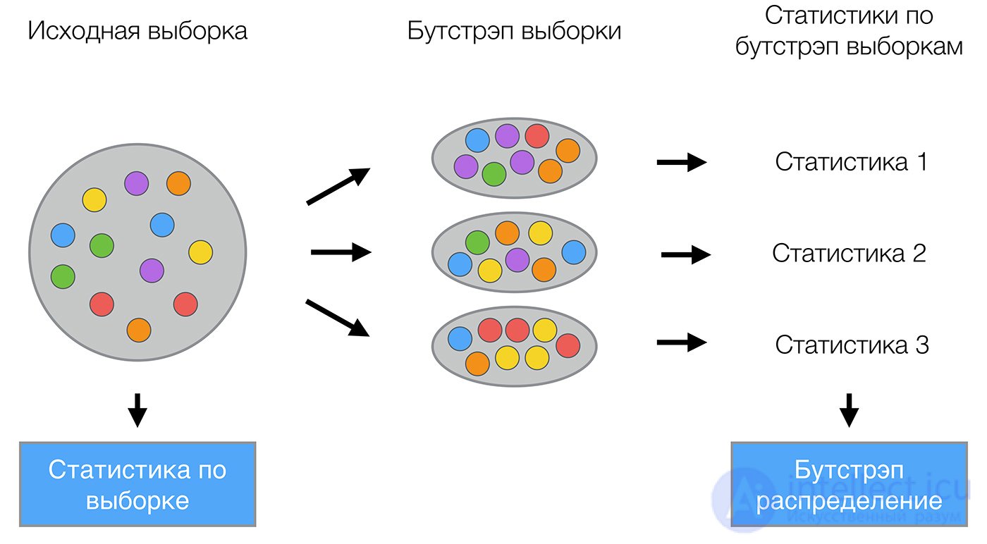
Bagging (from Bootstrap aggregation) is one of the first and simplest types of ensembles. It was invented by Leo Breiman in 1994. Bagging is based on the statistical bootstrap method, which makes it possible to estimate many statistics of complex distributions.
The bootstrap method works as follows. Suppose we have a sample  of size . Let's uniformly draw objects from the sample with replacement. This means that we will times pick an arbitrary object from the sample (assuming that each object is «picked» with equal probability
  ), and each time we choose from all the original objects. You can imagine a bag from which balls are drawn: a ball chosen at some step is put back into the bag, and the next draw is again made with equal probability from the same number of balls. Note that because of replacement, there will be repeats among them. Let's denote the new sample as
  . Repeating the procedure
  times, we generate subsamples
  . Now we have a sufficiently large number of samples and can estimate various statistics of the original distribution.
For example, let's take the telecom_churn dataset, which you already know from previous lessons of our course. Recall that this is a binary classification task for customer churn. One of the most important features in this dataset is the number of calls to the service center made by the customer. Let's try to visualize the data and look at the distribution of this feature.
Code for loading the data and building the plot
import pandas as pd
from matplotlib import pyplot as plt
plt.style.use('ggplot')
plt.rcParams['figure.figsize'] = 10, 6
import seaborn as sns
%matplotlib inline

telecom_data = pd.read_csv('data/telecom_churn.csv')

fig = sns.kdeplot(telecom_data[telecom_data['Churn'] == False]['Customer service calls'], label = 'Loyal')
fig = sns.kdeplot(telecom_data[telecom_data['Churn'] == True]['Customer service calls'], label = 'Churn')
fig.set(xlabel='Number of calls', ylabel='Density')
plt.show()
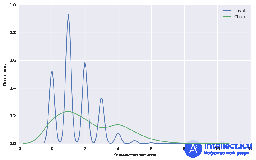
As you may have already noticed, the number of calls to the service center is lower for loyal customers than for our former customers. Now it would be good to estimate how many calls each of the groups makes on average. Since there is little data in our dataset, computing the mean directly isn't quite correct; it's better to apply our new bootstrap knowledge. Let's generate 1000 new subsamples from our population and make an interval estimate of the mean.
Code for constructing a confidence interval using the bootstrap
import numpy as np
def get_bootstrap_samples(data, n_samples):
    # function for generating subsamples using the bootstrap
    indices = np.random.randint(0, len(data), (n_samples, len(data)))
    samples = data[indices]
    return samples
def stat_intervals(stat, alpha):
    # function for interval estimation
    boundaries = np.percentile(stat, [100 * alpha / 2., 100 * (1 - alpha / 2.)])
    return boundaries

# save data for loyal and already churned customers into separate numpy arrays
loyal_calls = telecom_data[telecom_data['Churn'] == False]['Customer service calls'].values
churn_calls= telecom_data[telecom_data['Churn'] == True]['Customer service calls'].values

# set seed for reproducibility of results
np.random.seed(0)

# generate samples using the bootstrap and immediately compute the mean for each of them
loyal_mean_scores = [np.mean(sample)
                       for sample in get_bootstrap_samples(loyal_calls, 1000)]
churn_mean_scores = [np.mean(sample)
                       for sample in get_bootstrap_samples(churn_calls, 1000)]

#  print the interval estimate of the mean
print("Service calls from loyal:  mean interval",  stat_intervals(loyal_mean_scores, 0.05))
print("Service calls from churn:  mean interval",  stat_intervals(churn_mean_scores, 0.05))
As a result, we found that with 95% probability the average number of calls from loyal customers lies between 1.40 and 1.50, while our former customers called on average between 2.06 and 2.40 times. It's also worth noting that the interval for loyal customers is narrower, which makes sense, since they call rarely (mostly 0, 1, or 2 times), while dissatisfied customers call much more often, but eventually their patience runs out and they switch operators.
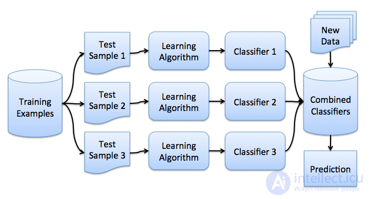
Now you have an idea of the bootstrap, and we can move on directly to bagging. Suppose we have a training sample . Using the bootstrap, let's generate samples from it. Now on each sample we train our own classifier  . The final classifier will average the responses of all these algorithms (in the case of classification, this corresponds to voting):
 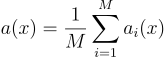 . This scheme can be represented by the picture below.
Let's consider a regression problem with base algorithms  . Suppose that there exists a true response function for all objects
  , and a distribution over the objects
  is also given. In this case, we can write the error of each regression function

and write the expected value of the mean squared error

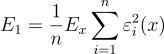
The average error of the constructed regression functions has the form
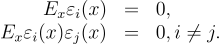
Assume that the errors are unbiased and uncorrelated:
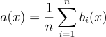
Let's now construct a new regression function that will average the answers of the functions we built:
Let's find its mean squared error:
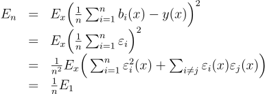
Thus, averaging the answers allowed us to reduce the mean squared error by a factor of n!
Let's recall from our previous lesson how the total error decomposes:
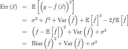
Bagging makes it possible to reduce the variance of the trained classifier, reducing the extent to which the error will differ depending on which dataset the model is trained on — in other words, it prevents overfitting. The effectiveness of bagging is achieved because the base algorithms, trained on different subsamples, turn out to be sufficiently different, and their errors mutually compensate for each other during voting, as well as due to the fact that outlier objects may not end up in some of the training subsamples.
The scikit-learn library has implementations of BaggingRegressor and BaggingClassifier, which allow using most other algorithms "inside". Let's look at how bagging works in practice, and compare it with a decision tree, using an example from the documentation.
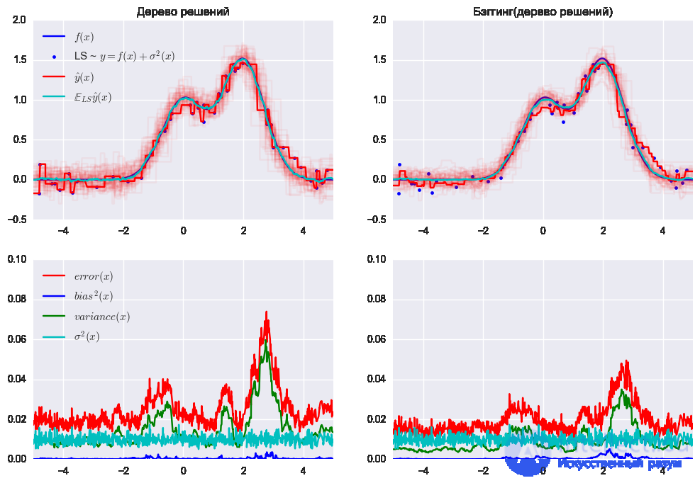
Decision tree error

Bagging error

The graph and the results above show that the variance error is much smaller with bagging, as we proved theoretically above.
Bagging is effective on small samples, where excluding even a small part of the training objects leads to building substantially different base classifiers. In the case of large samples, subsamples of substantially smaller length are usually generated.
It should be noted that the example we considered is not very applicable in practice, since we assumed that the errors are uncorrelated, which is rarely the case. If this assumption is false, the reduction in error turns out to be less significant. In the following lectures we will look at more sophisticated methods of combining algorithms into a composition, which make it possible to achieve high quality on real-world tasks.
Looking ahead, let's note that when using random forests there is no need for cross-validation or a separate test set to obtain an unbiased estimate of the test set error. Let's see how an "internal" estimate of the model is obtained during its training.
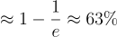
Each tree is built using different bootstrap samples from the original data. Approximately 37% of the examples are left out of the bootstrap sample and are not used when building the k-th tree.
This can easily be proved: suppose there are  objects in the sample. At each step, all objects fall into the subsample with replacement with equal probability, i.e. a specific object — with probability
  The probability that an object will NOT end up in the subsample (i.e. it was not picked times):
  . As
. As  we get one of the "remarkable" limits
  . Then the probability of a specific object ending up in the subsample is
  .
.
Let's look at how this works in practice:
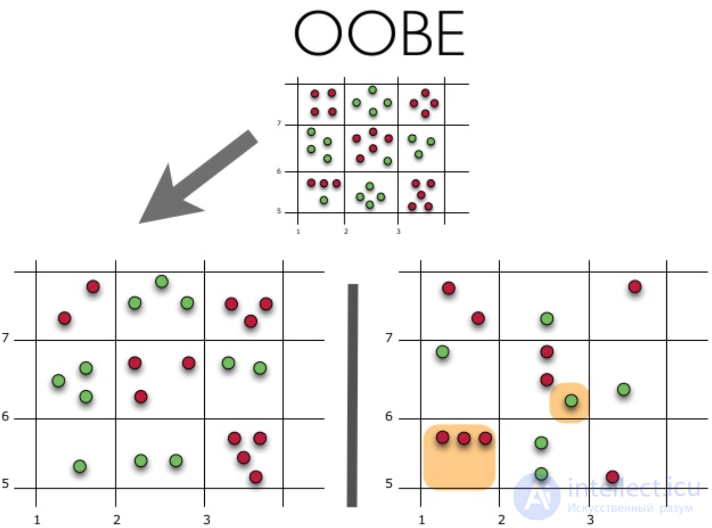
The figure shows an estimate of the oob error. The top figure is our original sample, which we split into training (on the left) and test (on the right). In the figure on the left we have a grid of small squares that perfectly partitions our sample. Now we need to estimate the fraction of correct answers on our test sample. The figure shows that our classifier made mistakes on 4 observations that we did not use for training. This means the fraction of correct answers of our classifier is: 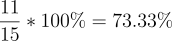
It turns out that each base algorithm is trained on ~63% of the original objects. This means that it can immediately be validated on the remaining ~37%. The Out-of-Bag estimate is the averaged estimate of the base algorithms on the ~37% of data on which they were not trained.
Leo Breiman found a use for the bootstrap not only in statistics, but also in machine learning. Together with Adele Cutler, he improved the random forest algorithm proposed by Ho, adding to the original version the construction of uncorrelated trees based on CART, combined with the random subspace method and bagging.
Decision trees are a good family of base classifiers for bagging, since they are sufficiently complex and can achieve zero error on any sample. The random subspace method makes it possible to reduce the correlation between trees and avoid overfitting. Base algorithms are trained on different subsets of the feature description, which are also selected at random.
An ensemble of models using the random subspace method can be built using the following algorithm:
, and the number of features  .
. as the number of individual models in the ensemble.
 choose
  as the number of features for . Usually only one value
  is used for all models. create a training set by selecting features from , and train the model.models by majority voting or by combining the posterior probabilities.
The algorithm for building a random forest consisting of trees looks as follows:
 :
:
 using the bootstrap;
 on the sample :
 objects, or until we reach a certain tree height random features out of the original
  are first selected,
The final classifier 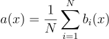 , in simple terms — for a classification task we choose the decision by majority vote, and for a regression task — by the mean.
It is recommended to take  for classification tasks, and
  for regression tasks, where is the number of features. It is also recommended, for classification tasks, to build each tree until each leaf contains a single object, and for regression tasks, until each leaf contains five objects.
Thus, a random forest is bagging over decision trees, in which, for each split during training, features are chosen from a certain random subset of features.
Code for comparing a decision tree, bagging, and a random forest for a regression task
from __future__ import division, print_function
# turn off all Anaconda warnings
import warnings
warnings.filterwarnings('ignore')
%pylab inline
np.random.seed(42)
figsize(8, 6)
import seaborn as sns
from sklearn.ensemble import RandomForestRegressor, RandomForestClassifier, BaggingRegressor
from sklearn.tree import DecisionTreeRegressor, DecisionTreeClassifier

n_train = 150
n_test = 1000
noise = 0.1

# Generate data
def f(x):
    x = x.ravel()
    return np.exp(-x ** 2) + 1.5 * np.exp(-(x - 2) ** 2)

def generate(n_samples, noise):
    X = np.random.rand(n_samples) * 10 - 5
    X = np.sort(X).ravel()
    y = np.exp(-X ** 2) + 1.5 * np.exp(-(X - 2) ** 2)\
        + np.random.normal(0.0, noise, n_samples)
    X = X.reshape((n_samples, 1))

    return X, y

X_train, y_train = generate(n_samples=n_train, noise=noise)
X_test, y_test = generate(n_samples=n_test, noise=noise)

# One decision tree regressor
dtree = DecisionTreeRegressor().fit(X_train, y_train)
d_predict = dtree.predict(X_test)

plt.figure(figsize=(10, 6))
plt.plot(X_test, f(X_test), "b")
plt.scatter(X_train, y_train, c="b", s=20)
plt.plot(X_test, d_predict, "g", lw=2)
plt.xlim([-5, 5])
plt.title("Decision tree, MSE = %.2f"
          % np.sum((y_test - d_predict) ** 2))

# Bagging decision tree regressor
bdt = BaggingRegressor(DecisionTreeRegressor()).fit(X_train, y_train)
bdt_predict = bdt.predict(X_test)

plt.figure(figsize=(10, 6))
plt.plot(X_test, f(X_test), "b")
plt.scatter(X_train, y_train, c="b", s=20)
plt.plot(X_test, bdt_predict, "y", lw=2)
plt.xlim([-5, 5])
plt.title("Bagging of decision trees, MSE = %.2f" % np.sum((y_test - bdt_predict) ** 2));

# Random Forest
rf = RandomForestRegressor(n_estimators=10).fit(X_train, y_train)
rf_predict = rf.predict(X_test)

plt.figure(figsize=(10, 6))
plt.plot(X_test, f(X_test), "b")
plt.scatter(X_train, y_train, c="b", s=20)
plt.plot(X_test, rf_predict, "r", lw=2)
plt.xlim([-5, 5])
plt.title("Random forest, MSE = %.2f" % np.sum((y_test - rf_predict) ** 2));
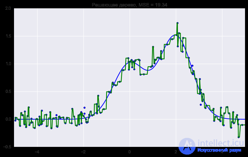
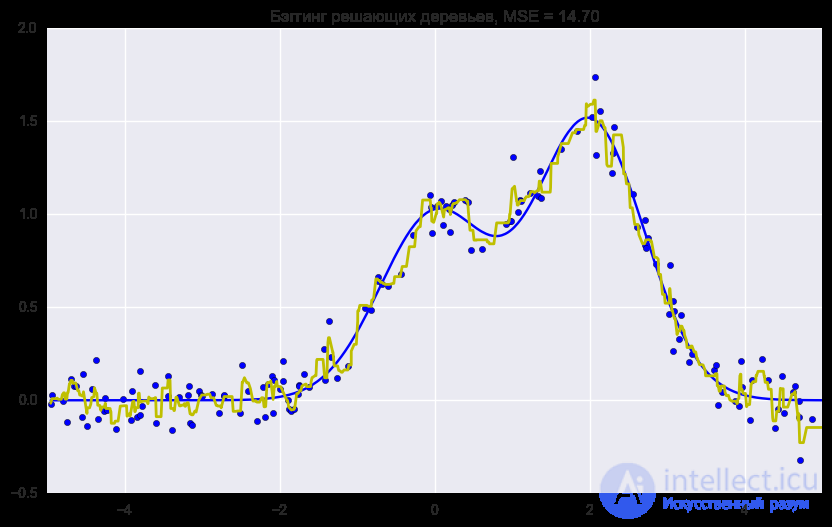
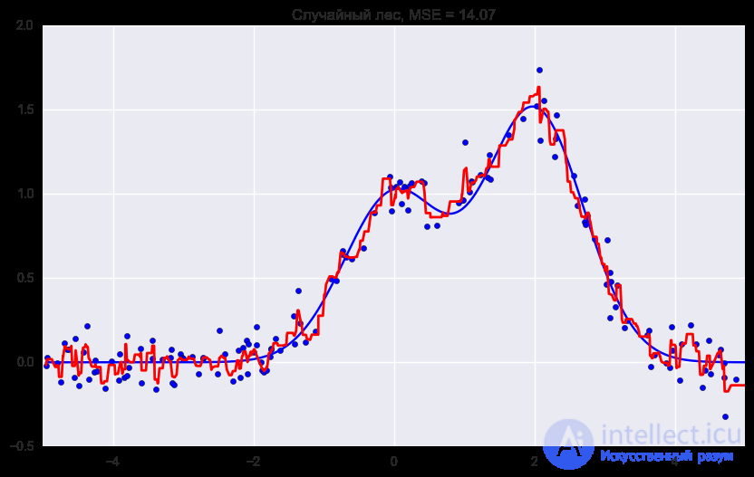
As we can see from the graphs and the MSE error values, a random forest of 10 trees gives a better result than a single tree or a bagging ensemble of 10 decision trees. The main difference between random forest and bagging on decision trees is that in random forest a random subset of features is selected, and the best feature for splitting a node is determined from a subsample of features, unlike bagging, where all features are considered for splitting at the node.
The advantage of random forest and bagging can also be seen in classification tasks.
Code for comparing a decision tree, bagging, and a random forest for a classification task
from sklearn.ensemble import RandomForestClassifier, BaggingClassifier
from sklearn.tree import DecisionTreeClassifier
from sklearn.datasets import make_circles
from sklearn.cross_validation import train_test_split
import numpy as np
from matplotlib import pyplot as plt
plt.style.use('ggplot')
plt.rcParams['figure.figsize'] = 10, 6
%matplotlib inline

np.random.seed(42)
X, y = make_circles(n_samples=500, factor=0.1, noise=0.35, random_state=42)
X_train_circles, X_test_circles, y_train_circles, y_test_circles = train_test_split(X, y, test_size=0.2)

dtree = DecisionTreeClassifier(random_state=42)
dtree.fit(X_train_circles, y_train_circles)

x_range = np.linspace(X.min(), X.max(), 100)
xx1, xx2 = np.meshgrid(x_range, x_range)
y_hat = dtree.predict(np.c_[xx1.ravel(), xx2.ravel()])
y_hat = y_hat.reshape(xx1.shape)
plt.contourf(xx1, xx2, y_hat, alpha=0.2)
plt.scatter(X[:,0], X[:,1], c=y, cmap='autumn')
plt.title("Decision tree")
plt.show()

b_dtree = BaggingClassifier(DecisionTreeClassifier(),n_estimators=300, random_state=42)
b_dtree.fit(X_train_circles, y_train_circles)

x_range = np.linspace(X.min(), X.max(), 100)
xx1, xx2 = np.meshgrid(x_range, x_range)
y_hat = b_dtree.predict(np.c_[xx1.ravel(), xx2.ravel()])
y_hat = y_hat.reshape(xx1.shape)
plt.contourf(xx1, xx2, y_hat, alpha=0.2)
plt.scatter(X[:,0], X[:,1], c=y, cmap='autumn')
plt.title("Bagging (decision tree)")
plt.show()

rf = RandomForestClassifier(n_estimators=300, random_state=42)
rf.fit(X_train_circles, y_train_circles)

x_range = np.linspace(X.min(), X.max(), 100)
xx1, xx2 = np.meshgrid(x_range, x_range)
y_hat = rf.predict(np.c_[xx1.ravel(), xx2.ravel()])
y_hat = y_hat.reshape(xx1.shape)
plt.contourf(xx1, xx2, y_hat, alpha=0.2)
plt.scatter(X[:,0], X[:,1], c=y, cmap='autumn')
plt.title("Random forest")
plt.show()
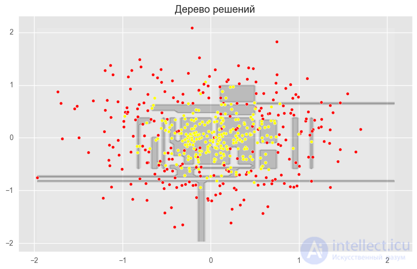
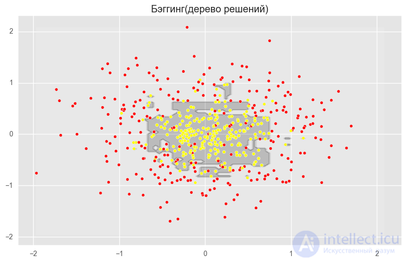
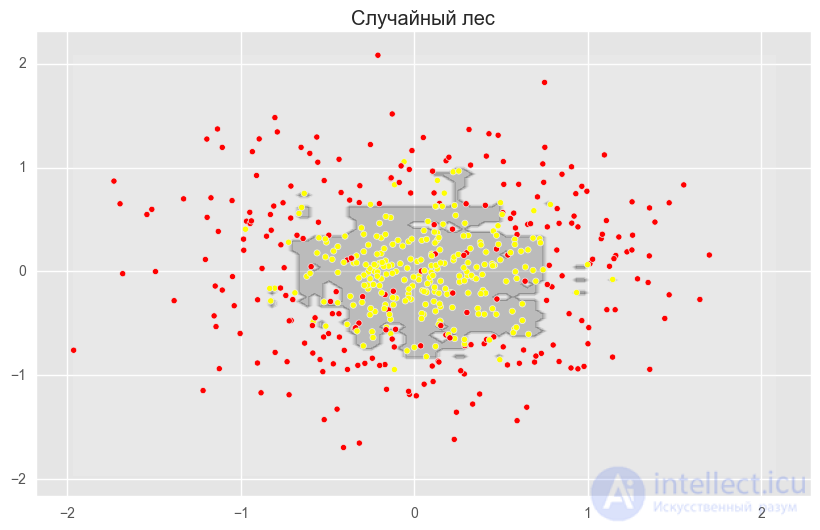
The figures above show that the decision boundary of the decision tree is very «jagged» and has many sharp angles, which indicates overfitting and poor generalization ability. Meanwhile, the boundary for bagging and random forest is fairly smooth, and there are practically no signs of overfitting.
Let's now try to figure out the parameters, by adjusting which we can increase the fraction of correct answers.
The random forest method is implemented in the scikit-learn machine learning library by two classes, RandomForestClassifier and RandomForestRegressor.
Full list of random forest parameters for the regression task:
class sklearn.ensemble.RandomForestRegressor(
    n_estimators — the number of trees in the "forest" (default – 10)
    criterion — the function that measures the quality of a branch split in the tree (default — "mse", "mae" can also be chosen)
    max_features — the number of features considered when looking for a split. You can specify a specific number or percentage of features, or choose from the available values: "auto" (all features), "sqrt", "log2". The default is "auto".
    max_depth — the maximum depth of the tree (by default the depth is unlimited)
    min_samples_split — the minimum number of objects required to split an internal node. Can be set as a number or a percentage of the total number of objects (default — 2)
    min_samples_leaf — the minimum number of objects in a leaf. Can be set as a number or a percentage of the total number of objects (default — 1)
    min_weight_fraction_leaf — the minimum weighted fraction of the total sum of weights (of all input objects) that must be in a leaf (by default they have equal weight)
    max_leaf_nodes — the maximum number of leaves (by default there is no limit)
    min_impurity_split — threshold for stopping the growth of the tree (default 1e-7)
    bootstrap — whether to use the bootstrap for building the tree (default True)
    oob_score — whether to use out-of-bag objects to estimate R^2 (default False)
    n_jobs — the number of cores for building the model and making predictions (default 1; if set to -1, all cores will be used)
    random_state — the seed value for random number generation (by default there is none; if you want reproducible results, specify any int value
    verbose — output of logs during tree building (default 0)
    warm_start — uses an already trained model and adds trees to the ensemble (default False)
)
For the classification task everything is almost the same; we will only list the parameters by which RandomForestClassifier differs from RandomForestRegressor
class sklearn.ensemble.RandomForestClassifier(
    criterion — since we now have a classification task, the default criterion chosen is "gini" (you can choose "entropy")
    class_weight — the weight of each class (by default all weights are equal to 1, but you can pass a dictionary of weights, or explicitly specify "balanced", in which case the class weights will be equal to their original proportions in the population; you can also specify "balanced_subsample", in which case the weights on each subsample will change depending on the class distribution in that subsample.
)
Next, let's look at a few parameters that are worth paying attention to first when building a model:
Let's look at applying random forest to a real-world task
For this we will use the example with the customer churn task. This is a classification task, so we will use the accuracy metric to evaluate model quality. First, let's build the simplest classifier, which will be our baseline. We'll take only numerical features for simplicity.
Code for building a baseline for random forest
import pandas as pd
from sklearn.model_selection import cross_val_score, StratifiedKFold, GridSearchCV
from sklearn.metrics import accuracy_score

# Load the data
df = pd.read_csv("../../data/telecom_churn.csv")

# First select only the columns with numeric data types
cols = []
for i in df.columns:
    if (df[i].dtype == "float64") or (df[i].dtype == 'int64'):
        cols.append(i)

# Split into features and objects
X, y = df[cols].copy(), np.asarray(df["Churn"],dtype='int8')

# Initialize the stratified split of our dataset for validation
skf = StratifiedKFold(n_splits=5, shuffle=True, random_state=42)

# Initialize our classifier with default parameters
rfc = RandomForestClassifier(random_state=42, n_jobs=-1, oob_score=True)

# Train on the training dataset
results = cross_val_score(rfc, X, y, cv=skf)

# Evaluate the fraction of correct answers on the test dataset
print("CV accuracy score: {:.2f}%".format(results.mean()*100))
We got a fraction of correct answers of 91.21%; now let's try to improve this result and see how the validation curves behave as we change the main parameters.
Let's start with the number of trees:
Code for plotting validation curves for tuning the number of trees
# Initialize the validation
skf = StratifiedKFold(n_splits=5, shuffle=True, random_state=42)

# Create lists to store accuracy on the training and test datasets
train_acc = []
test_acc = []
temp_train_acc = []
temp_test_acc = []
trees_grid = [5, 10, 15, 20, 30, 50, 75, 100]

# Train on the training dataset
for ntrees in trees_grid:
    rfc = RandomForestClassifier(n_estimators=ntrees, random_state=42, n_jobs=-1, oob_score=True)
    temp_train_acc = []
    temp_test_acc = []
    for train_index, test_index in skf.split(X, y):
        X_train, X_test = X.iloc[train_index], X.iloc[test_index]
        y_train, y_test = y[train_index], y[test_index]
        rfc.fit(X_train, y_train)
        temp_train_acc.append(rfc.score(X_train, y_train))
        temp_test_acc.append(rfc.score(X_test, y_test))
    train_acc.append(temp_train_acc)
    test_acc.append(temp_test_acc)

train_acc, test_acc = np.asarray(train_acc), np.asarray(test_acc)
print("Best accuracy on CV is {:.2f}% with {} trees".format(max(test_acc.mean(axis=1))*100,
                                                        trees_grid[np.argmax(test_acc.mean(axis=1))]))
Code for plotting the validation curves graph
import matplotlib.pyplot as plt
plt.style.use('ggplot')
%matplotlib inline

fig, ax = plt.subplots(figsize=(8, 4))
ax.plot(trees_grid, train_acc.mean(axis=1), alpha=0.5, color='blue', label='train')
ax.plot(trees_grid, test_acc.mean(axis=1), alpha=0.5, color='red', label='cv')
ax.fill_between(trees_grid, test_acc.mean(axis=1) - test_acc.std(axis=1), test_acc.mean(axis=1) + test_acc.std(axis=1), color='#888888', alpha=0.4)
ax.fill_between(trees_grid, test_acc.mean(axis=1) - 2*test_acc.std(axis=1), test_acc.mean(axis=1) + 2*test_acc.std(axis=1), color='#888888', alpha=0.2)
ax.legend(loc='best')
ax.set_ylim([0.88,1.02])
ax.set_ylabel("Accuracy")
ax.set_xlabel("N_estimators")
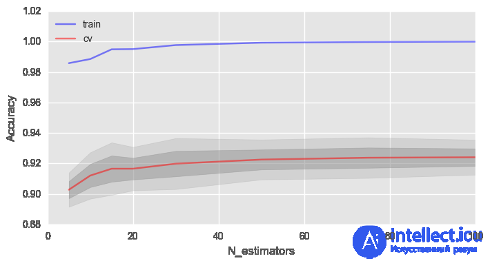
As you can see, once a certain number of trees is reached, our fraction of correct answers on the test set levels off to an asymptote, and you can decide for yourself how many trees are optimal for your task.
The figure also shows that on the training set we managed to achieve 100% accuracy, which tells us that our model is overfitting. To avoid overfitting, we need to add regularization parameters to the model.
Let's start with the maximum depth parameter – max_depth. (let's fix the number of trees at 100)
Code for plotting the learning curves for tuning the maximum tree depth
# Create lists to store accuracy on the training and test datasets
train_acc = []
test_acc = []
temp_train_acc = []
temp_test_acc = []
max_depth_grid = [3, 5, 7, 9, 11, 13, 15, 17, 20, 22, 24]

# Train on the training dataset
for max_depth in max_depth_grid:
    rfc = RandomForestClassifier(n_estimators=100, random_state=42, n_jobs=-1, oob_score=True, max_depth=max_depth)
    temp_train_acc = []
    temp_test_acc = []
    for train_index, test_index in skf.split(X, y):
        X_train, X_test = X.iloc[train_index], X.iloc[test_index]
        y_train, y_test = y[train_index], y[test_index]
        rfc.fit(X_train, y_train)
        temp_train_acc.append(rfc.score(X_train, y_train))
        temp_test_acc.append(rfc.score(X_test, y_test))
    train_acc.append(temp_train_acc)
    test_acc.append(temp_test_acc)

train_acc, test_acc = np.asarray(train_acc), np.asarray(test_acc)
print("Best accuracy on CV is {:.2f}% with {} max_depth".format(max(test_acc.mean(axis=1))*100,
                                                        max_depth_grid[np.argmax(test_acc.mean(axis=1))]))
Code for plotting the learning curves graph
fig, ax = plt.subplots(figsize=(8, 4))
ax.plot(max_depth_grid, train_acc.mean(axis=1), alpha=0.5, color='blue', label='train')
ax.plot(max_depth_grid, test_acc.mean(axis=1), alpha=0.5, color='red', label='cv')
ax.fill_between(max_depth_grid, test_acc.mean(axis=1) - test_acc.std(axis=1), test_acc.mean(axis=1) + test_acc.std(axis=1), color='#888888', alpha=0.4)
ax.fill_between(max_depth_grid, test_acc.mean(axis=1) - 2*test_acc.std(axis=1), test_acc.mean(axis=1) + 2*test_acc.std(axis=1), color='#888888', alpha=0.2)
ax.legend(loc='best')
ax.set_ylim([0.88,1.02])
ax.set_ylabel("Accuracy")
ax.set_xlabel("Max_depth")
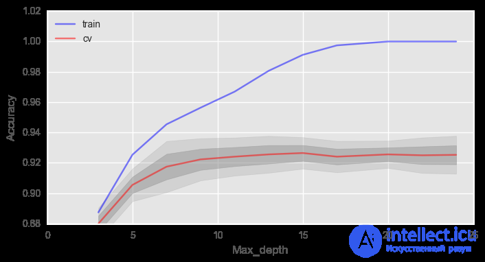
The max_depth parameter handles the model's regularization well, and we are no longer overfitting as strongly. The fraction of correct answers of our model has increased slightly.
Another important parameter is min_samples_leaf, which also acts as a regularizer.
Code for plotting validation curves for tuning the minimum number of samples in a tree leaf
# Create lists to store accuracy on the training and test datasets
train_acc = []
test_acc = []
temp_train_acc = []
temp_test_acc = []
min_samples_leaf_grid = [1, 3, 5, 7, 9, 11, 13, 15, 17, 20, 22, 24]

# Train on the training dataset
for min_samples_leaf in min_samples_leaf_grid:
    rfc = RandomForestClassifier(n_estimators=100, random_state=42, n_jobs=-1,
                                 oob_score=True, min_samples_leaf=min_samples_leaf)
    temp_train_acc = []
    temp_test_acc = []
    for train_index, test_index in skf.split(X, y):
        X_train, X_test = X.iloc[train_index], X.iloc[test_index]
        y_train, y_test = y[train_index], y[test_index]
        rfc.fit(X_train, y_train)
        temp_train_acc.append(rfc.score(X_train, y_train))
        temp_test_acc.append(rfc.score(X_test, y_test))
    train_acc.append(temp_train_acc)
    test_acc.append(temp_test_acc)

train_acc, test_acc = np.asarray(train_acc), np.asarray(test_acc)
print("Best accuracy on CV is {:.2f}% with {} min_samples_leaf".format(max(test_acc.mean(axis=1))*100,
                                                        min_samples_leaf_grid[np.argmax(test_acc.mean(axis=1))]))
Code for plotting the validation curves graph
fig, ax = plt.subplots(figsize=(8, 4))
ax.plot(min_samples_leaf_grid, train_acc.mean(axis=1), alpha=0.5, color='blue', label='train')
ax.plot(min_samples_leaf_grid, test_acc.mean(axis=1), alpha=0.5, color='red', label='cv')
ax.fill_between(min_samples_leaf_grid, test_acc.mean(axis=1) - test_acc.std(axis=1), test_acc.mean(axis=1) + test_acc.std(axis=1), color='#888888', alpha=0.4)
ax.fill_between(min_samples_leaf_grid, test_acc.mean(axis=1) - 2*test_acc.std(axis=1), test_acc.mean(axis=1) + 2*test_acc.std(axis=1), color='#888888', alpha=0.2)
ax.legend(loc='best')
ax.set_ylim([0.88,1.02])
ax.set_ylabel("Accuracy")
ax.set_xlabel("Min_samples_leaf")
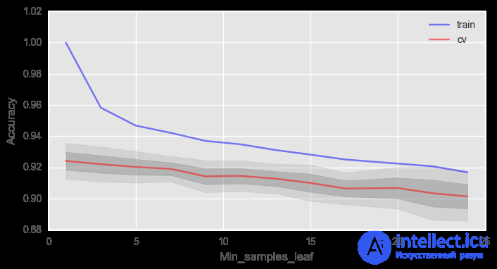
In this case we don't gain anything in validation accuracy, but we can significantly reduce overfitting to 2% while keeping accuracy around 92%.
Let's consider a parameter such as max_features. For classification tasks,  is used by default, where n is the number of features. Let's check whether it is optimal in our case to use 4 features or not.
Code for plotting validation curves for tuning the maximum number of features for a single tree
# Create lists to store accuracy on the training and test datasets
train_acc = []
test_acc = []
temp_train_acc = []
temp_test_acc = []
max_features_grid = [2, 4, 6, 8, 10, 12, 14, 16]

# Train on the training dataset
for max_features in max_features_grid:
    rfc = RandomForestClassifier(n_estimators=100, random_state=42, n_jobs=-1,
                                 oob_score=True, max_features=max_features)
    temp_train_acc = []
    temp_test_acc = []
    for train_index, test_index in skf.split(X, y):
        X_train, X_test = X.iloc[train_index], X.iloc[test_index]
        y_train, y_test = y[train_index], y[test_index]
        rfc.fit(X_train, y_train)
        temp_train_acc.append(rfc.score(X_train, y_train))
        temp_test_acc.append(rfc.score(X_test, y_test))
    train_acc.append(temp_train_acc)
    test_acc.append(temp_test_acc)

train_acc, test_acc = np.asarray(train_acc), np.asarray(test_acc)
print("Best accuracy on CV is {:.2f}% with {} max_features".format(max(test_acc.mean(axis=1))*100,
                                                        max_features_grid[np.argmax(test_acc.mean(axis=1))]))
Code for plotting the validation curves graph
fig, ax = plt.subplots(figsize=(8, 4))
ax.plot(max_features_grid, train_acc.mean(axis=1), alpha=0.5, color='blue', label='train')
ax.plot(max_features_grid, test_acc.mean(axis=1), alpha=0.5, color='red', label='cv')
ax.fill_between(max_features_grid, test_acc.mean(axis=1) - test_acc.std(axis=1), test_acc.mean(axis=1) + test_acc.std(axis=1), color='#888888', alpha=0.4)
ax.fill_between(max_features_grid, test_acc.mean(axis=1) - 2*test_acc.std(axis=1), test_acc.mean(axis=1) + 2*test_acc.std(axis=1), color='#888888', alpha=0.2)
ax.legend(loc='best')
ax.set_ylim([0.88,1.02])
ax.set_ylabel("Accuracy")
ax.set_xlabel("Max_features")
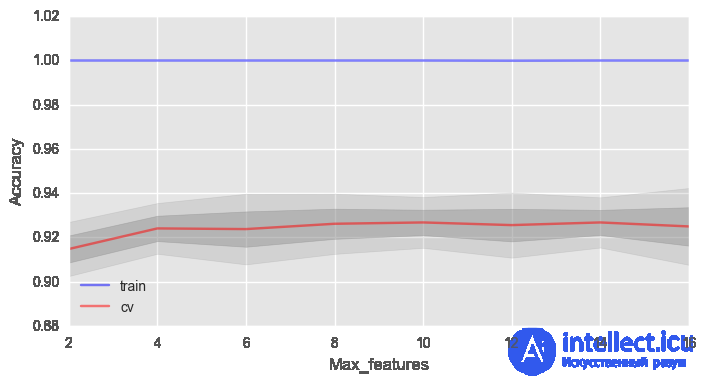
In our case, the optimal number of features is 10 — this is exactly the value at which the best result is achieved.
We have looked at how the validation curves behave depending on changes in the main parameters. Now let's use GridSearchCV to find the optimal parameters for our example.
Code for tuning the model's optimal parameters
# Initialize the parameters over which we want to do a full grid search
parameters = {'max_features': [4, 7, 10, 13], 'min_samples_leaf': [1, 3, 5, 7], 'max_depth': [5,10,15,20]}
rfc = RandomForestClassifier(n_estimators=100, random_state=42,
                             n_jobs=-1, oob_score=True)
gcv = GridSearchCV(rfc, parameters, n_jobs=-1, cv=skf, verbose=1)
gcv.fit(X, y)
The best fraction of correct answers we managed to achieve through the parameter search is 92.83% with 'max_depth': 15, 'max_features': 7, 'min_samples_leaf': 3.
Let's write the variance for a random forest as

Here
 – the sample correlation between any two trees used in averaging

 and
and  – a randomly selected pair of trees on randomly selected sample objects
 — is the sample variance of any arbitrarily chosen tree:

It is easy to confuse  with the average correlation between the trained trees in this random forest, by treating the trees as N-vectors and computing the average pairwise correlation between them. This is not the case. This conditional correlation has no direct relation to the averaging process, and the dependence on
  in warns us of this distinction. Rather, is the theoretical correlation between a pair of random trees, evaluated at the point , which arose from repeatedly sampling the training set from the population , after which this pair of random trees was selected. In statistical jargon, this is a correlation induced by the sampling distribution of and
  .
.
In fact, the conditional covariance of a pair of trees is 0, because bootstrapping and feature selection are independent and identically distributed.
If we look at the variance of a single tree, it barely changes with the splitting variables (), but for an ensemble this plays a big role, and the variance for a tree is much higher than for an ensemble.
The book The Elements of Statistical Learning (Trevor Hastie, Robert Tibshirani and Jerome Friedman) has a great example that demonstrates this.
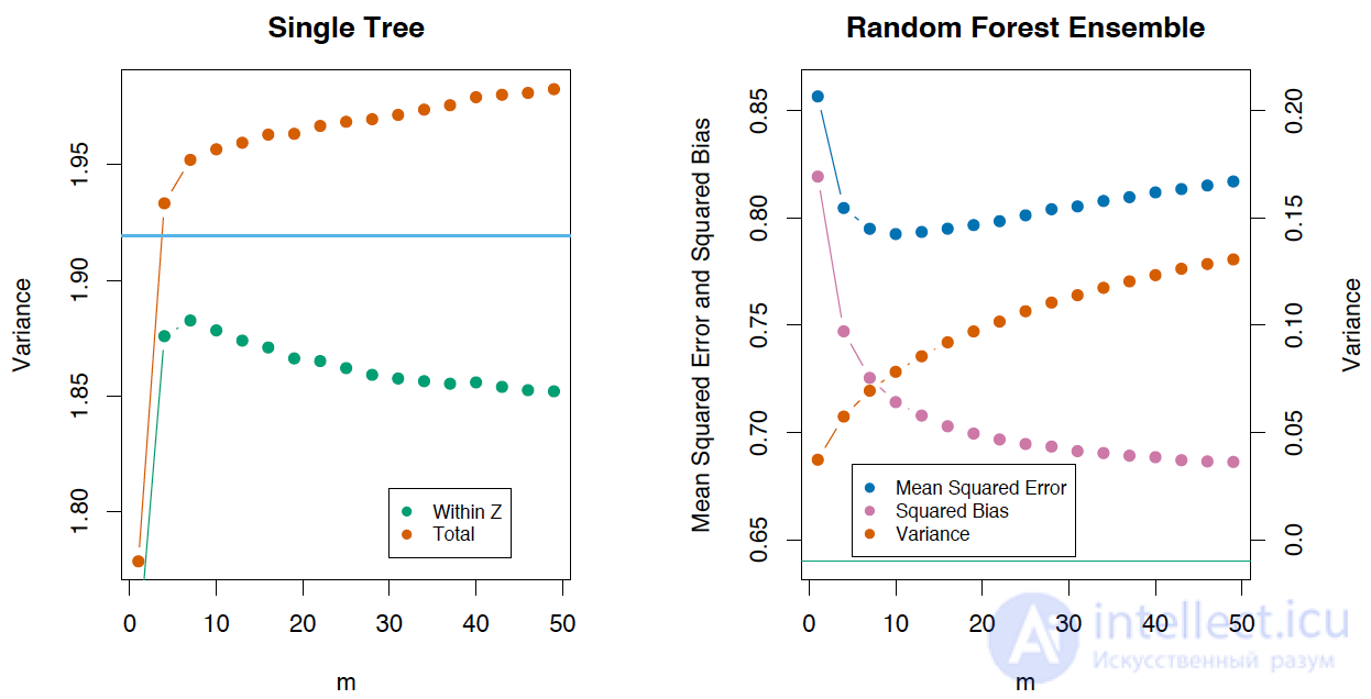
As in bagging, the bias in a random forest is the same as the bias of an individually taken tree  :
:

This is also usually larger (in absolute terms) than the bias of an «unprunned» tree, since randomization and shrinking the sample space impose constraints. Consequently, the improvements in prediction obtained through bagging or random forests are exclusively the result of variance reduction.
In Extremely Randomized Trees, there is more randomness in how the splits at the nodes are computed. As in random forests, a random subset of the possible features is used, but instead of searching for the most optimal thresholds, threshold values are chosen randomly for each possible feature, and the best of these randomly generated thresholds is chosen as the best rule for splitting the node. This usually allows a slight reduction in the model's variance at the cost of a somewhat larger increase in bias.
The scikit-learn library has an implementation of ExtraTreesClassifier and ExtraTreesRegressor. This method is worth using when you are strongly overfitting on a random forest or gradient boosting.
The random forest method is similar to the nearest neighbors method. Random forests, in essence, make predictions for objects based on the labels of similar objects from the training set. The similarity of objects is higher the more often these objects end up in the same leaf of a tree. Let's show this formally.
Let's consider a regression problem with a quadratic loss function. Let  be the number of the leaf of the
  -th tree of the random forest into which object falls. The answer for object is equal to the average answer over all training set objects that fell into this leaf . This can be written as
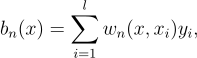
where


that the object falls into is by itself a valuable feature. An approach that works quite well is one where a composition of a small number of trees is trained on the sample using a random forest or gradient boosting, and then categorical features  are added to it. The new features are the result of a nonlinear partitioning of the space and carry information about the similarity of objects.
That same book, The Elements of Statistical Learning, has a good illustrative example of the similarity between a random forest and k-nearest neighbors.
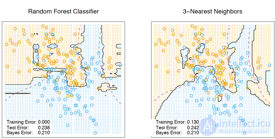
Everyone is used to using a random forest for supervised learning tasks, but it is also possible to use it for unsupervised learning. With the RandomTreesEmbedding method we can transform our dataset into a high-dimensional sparse representation of it. Its essence is that we build completely random trees, and we treat the index of the leaf that an observation ends up in as a new feature. If an object falls into the first leaf, we set 1, and if it doesn't, we set 0. This is the so-called binary encoding. We can control the number of variables as well as the sparsity of our new representation of the dataset by increasing/decreasing the number of trees and their depth. Since neighboring data points are likely to lie in the same leaf of a tree, the transformation performs an implicit, nonparametric density estimation.
Very often you want to understand your algorithm — why it gave a particular answer in this way and not another. Or, if you can't understand it fully, at least which variables have the greatest influence on the result. This information can be obtained quite easily from a random forest.
From this picture it is intuitively clear that the importance of the «Age» feature in a credit scoring problem is higher than the importance of the «Income» feature. This is formalized using the concept of information gain.
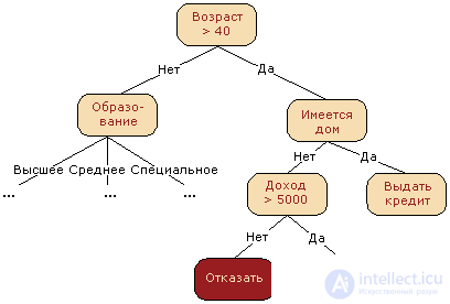
If you build many decision trees (a random forest), then the higher on average a feature is in a decision tree, the more important it is for the given classification/regression task. At each split in each tree, the improvement in the splitting criterion (in our case, Gini impurity) is an importance measure associated with the splitting variable, and it is accumulated across all the trees of the forest separately for each variable.
Let's go a bit deeper into the details. The average decrease in accuracy caused by a variable is determined during the out-of-bag error computation phase. The more the prediction accuracy decreases because of excluding (or permuting) a single variable, the more important that variable is, and so variables with a larger average decrease in accuracy are more important for classifying the data. The average decrease in Gini impurity (or mse error in regression problems) is a measure of how much each variable contributes to the homogeneity of the nodes and leaves in the final random forest model. Every time a particular variable is used to split a node, the Gini impurity for the child nodes is computed and compared with the impurity of the parent node. Gini impurity is a measure of homogeneity ranging from 0 (homogeneous) to 1 (heterogeneous). The changes in the value of the splitting criterion are summed for each variable and normalized at the end of the computation. Variables that lead to nodes with higher purity have a higher decrease in the Gini coefficient.
Now let's express everything described above in the form of formulas.

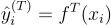 — the class prediction before permuting/removing the feature
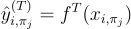 — the class prediction after permuting/removing the feature

Note that 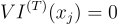 if
if  is not in tree
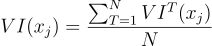
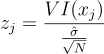
Calculation of feature importance in the ensemble:
— unnormalized
— normalized
Example
Let's consider the results of a survey of hostel guests from the Booking.com and TripAdvisor.com websites. The features are average scores for various factors (listed below) — staff, room condition, etc. The target feature is the hostel's rating on the website.
from __future__ import division, print_function
# turn off all sorts of Anaconda warnings
import warnings
warnings.filterwarnings('ignore')
%pylab inline
import seaborn as sns
# russian headres
from matplotlib import rc
font = {'family': 'Verdana',
        'weight': 'normal'}
rc('font', **font)
import pandas as pd
import numpy as np
from sklearn.ensemble.forest import RandomForestRegressor

hostel_data = pd.read_csv("../../data/hostel_factors.csv")
features = {"f1":u"Staff",
"f2":u"Hostel booking ",
"f3":u"Check-in and check-out",
"f4":u"Room condition",
"f5":u"Common kitchen condition",
"f6":u"Common space condition",
"f7":u"Additional services",
"f8":u"General conditions and amenities",
"f9":u"Price/quality",
"f10":u"ССЦ"}

forest = RandomForestRegressor(n_estimators=1000, max_features=10,
                                random_state=0)

forest.fit(hostel_data.drop(['hostel', 'rating'], axis=1),
           hostel_data['rating'])
importances = forest.feature_importances_

indices = np.argsort(importances)[::-1]
# Plot the feature importancies of the forest
num_to_plot = 10
feature_indices = [ind+1 for ind in indices[:num_to_plot]]

# Print the feature ranking
print("Feature ranking:")

for f in range(num_to_plot):
    print("%d. %s %f " % (f + 1,
            features["f"+str(feature_indices[f])],
            importances[indices[f]]))
plt.figure(figsize=(15,5))
plt.title(u"Importance of the constructs")
bars = plt.bar(range(num_to_plot),
               importances[indices[:num_to_plot]],
       color=([str(i/float(num_to_plot+1))
               for i in range(num_to_plot)]),
               align="center")
ticks = plt.xticks(range(num_to_plot),
                   feature_indices)
plt.xlim([-1, num_to_plot])
plt.legend(bars, [u''.join(features["f"+str(i)])
                  for i in feature_indices]);
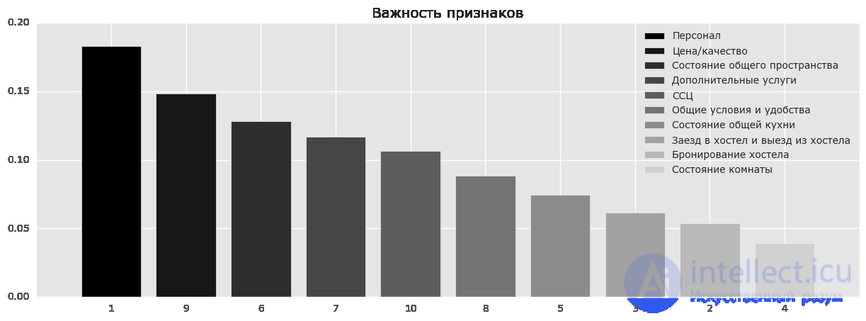
The figure above shows that people pay the most attention to the staff and the price/quality ratio, and they write their reviews based on the impression left by these things. But the difference between these features and the less influential ones is not very significant, and dropping some feature would lead to a decrease in the accuracy of our model. But even based on our analysis, we can give recommendations to hotels to primarily train the staff better and/or improve the quality up to the stated price.
Pros:
— has high prediction accuracy; on most tasks it will outperform linear algorithms, and its accuracy is comparable to that of boosting
— is practically insensitive to outliers in the data due to random sampling
— is insensitive to scaling (and in general to any monotonic transformations) of feature values, which is related to the choice of random subspaces
— does not require careful parameter tuning, and works well «out of the box». Through parameter «tuning», a gain of 0.5 to 3% in accuracy can be achieved, depending on the task and data
— is able to efficiently handle data with a large number of features and classes
— handles both continuous and discrete features equally well
— rarely overfits; in practice, adding trees almost always only improves the ensemble, but on validation, after reaching a certain number of trees, the learning curve levels off to an asymptote
— for a random forest there exist methods for assessing the significance of individual features in the model
— works well with missing data; retains good accuracy even if most of the data is missing
— allows the weight of each class to be balanced over the entire sample, or over the subsample of each tree
— computes the proximity between pairs of objects, which can be used for clustering, outlier detection, or (through scaling) provide interesting representations of the data
— the capabilities described above can be extended to unlabeled data, which makes it possible to perform clustering and visualization of the data, and to detect outliers
— high parallelizability and scalability.
Cons:
— unlike a single tree, the results of a random forest are harder to interpret
— there are no formal conclusions (p-values) available for assessing the importance of variables
— the algorithm performs worse than many linear methods when the sample has a lot of sparse features (texts, Bag of Words)
— a random forest cannot extrapolate, unlike, say, linear regression (but this can also be considered an advantage, since there will be no extreme values in the case of an outlier)
— the algorithm is prone to overfitting on some tasks, especially on noisy data
— for data that includes categorical variables with different numbers of levels, random forests are biased in favor of features with a larger number of levels: when a feature has many levels, the tree will fit more strongly to precisely those features, since a higher value of the optimized functional (such as information gain) can be obtained on them
— if the data contains groups of correlated features that have similar significance for the labels, then smaller groups are preferred over larger ones
— a larger size of the resulting models.  of memory is required to store the model, where
  is the number of trees.
Current homework assignments are announced during the next session of the course; you can follow them in the VK group and in the course repository.
To reinforce the material, we suggest completing this assignment – work through bagging and train random forest and logistic regression models to solve a credit scoring problem. You can check yourself by submitting your answers in the web form (you will also find the solution there).
– Open Machine Learning Course. Topic 5. Bagging and Random Forest (a translation of this article into English)
– A video recording of a lecture based on this article
– Section 15 of the book “Elements of Statistical Learning” by Jerome H. Friedman, Robert Tibshirani, and Trevor Hastie
– Alexander Dyakonov's blog
– More about the practical application of random forests and other ensemble algorithms in the official scikit-learn documentation
– Evgeny Sokolov's machine learning course (materials on GitHub). There are additional practical assignments to deepen your knowledge
– The survey article "History of the development of ensemble classification methods in machine learning" (Yu. Kashnitsky)

Comments