1. Exploratory Data Analysis with Pandas

. About the Course

We do not aim to create yet another comprehensive introductory course on machine learning or data analysis (that is, this is not a replacement for the Yandex and MIPT specialization, the HSE continuing education program, or other fundamental online and offline programs and books). The goal of this series of articles — to quickly refresh the knowledge you already have or help you find topics for further study. The approach is roughly the one taken by the authors of the book Deep Learning, which opens with an overview of mathematics and the foundations of machine learning — brief, as concise as possible, and rich in references to sources.

If you plan to take the course, be warned: when choosing topics and creating materials, we assume that our students know mathematics at the level of the 2nd year of a technical university and can at least program a little in Python. These are not strict admission criteria but merely recommendations — you can enroll in the course without knowing math or Python and catch up along the way:

• basic mathematics (calculus, linear algebra, optimization, probability theory and statistics) can be reviewed using these Yandex & MIPT lecture notes (shared with permission). Brief, in Russian – just what's needed. For a more detailed treatment: calculus – Kudryavtsev, linear algebra – Kostrikin, optimization – Boyd (in English), probability theory and statistics – Kibzun. Plus excellent online courses from MIPT and HSE on Coursera;
• for Python, a short interactive tutorial on Datacamp or this repository on Python and basic algorithms and data structures will suffice. Something more advanced – for example, the course from the St. Petersburg Computer Science Center;
• as for machine learning, there is the classic (though slightly outdated) course by Andrew Ng "Machine Learning"(Stanford, Coursera). In Russian, there is an excellent MIPT and Yandex specialization «Machine Learning and Data Analysis». And here are the best books: "Pattern recognition and Machine Learning" (Bishop), "Machine Learning: A Probabilistic Perspective " (Murphy), "The elements of statistical learning" (Hastie, Tibshirani, Friedman), "Deep Learning" (Goodfellow, Bengio, Courville). Goodfellow's book opens with an overview of mathematics and a clear and engaging introduction to machine learning and the inner workings of its algorithms. It's nice that there is now a book on deep learning in Russian too – "Deep Learning: A Journey into the World of Neural Networks" (Nikolenko S. I., Kadurin A. A., Arkhangelskaya E. O.).

Also, the course is covered in this announcement.

What software you need

To take the course, you need a number of Python packages, most of which are included in the Anaconda distribution with Python 3.6. A bit later you'll need other libraries too, which will be mentioned separately. The full list can be found in the Dockerfile.

You can also use a Docker container that already has all the necessary software installed. Details – on the repository's Wiki page.

How to join the course

No formal registration is required, you can join the course at any time after it starts (01.10.18 g.), but the homework deadlines are strict.
But so that we know more about you:

• Fill out the survey, providing your real full name;
• Join the OpenDataScience community, discussion of the course takes place in the #mlcourse.ai channel.

2. Homework Assignments in the Course

• Each article is accompanied by a homework assignment in the form of a Jupyter notebook, in which you need to add code, and based on that choose the correct answer in a Google form;
• Homework solutions are sent to those who submitted their solution through the form;
• At the end of the article series, the results will be summed up (a ranking of participants);
• Examples of homework assignments are given in the articles of the series (at the end).

3. Demonstration of the Main Pandas Methods

All the code can be reproduced in this Jupyter notebook.

Pandas — is a Python library that provides extensive capabilities for data analysis. The data that data scientists work with is often stored in the form of tables — for example, in .csv, .tsv, or .xlsx formats. With the Pandas library, such tabular data is very convenient to load, process, and analyze using SQL-like queries. And combined with the Matplotlib and Seaborn libraries, Pandas provides extensive capabilities for visual analysis of tabular data.

The main data structures in Pandas are the Series and DataFrame classes. The first of these is a one-dimensional indexed array of data of some fixed type. The second – is a two-dimensional data structure representing a table, each column of which contains data of a single type. You can think of it as a dictionary of Series objects. The DataFrame structure is well suited for representing real data: rows correspond to feature descriptions of individual objects, and columns correspond to features.

# import Pandas and Numpy
import pandas as pd
import numpy as np

We will demonstrate the main methods in action by analyzing a dataset on customer churn for a telecom operator (no need to download it, it's already in the repository). Let's read the data (the read_csv method) and look at the first 5 rows using the head method:

df = pd.read_csv('../../data/telecom_churn.csv')

df.head()

On displaying a dataframe in a Jupyter notebook

In Jupyter notebooks, Pandas dataframes are displayed as nice tables like this one, and print(df.head()) looks worse.
By default, Pandas displays only 20 columns and 60 rows, so if your dataframe is larger, use the set_option function:

pd.set_option('display.max_columns', 100)
pd.set_option('display.max_rows', 100)

Each row represents a single customer – this is the object of study.
Columns – are features of the object.

Description of features

Target variable: Churn – churn indicator, a binary feature (1 – customer loss, i.e. churn). Later we will build models that predict this feature from the others, which is why we called it the target.

Let's look at the size of the data, the names of the features, and their types.

print(df.shape)

(3333, 20)

We see that the table has 3333 rows and 20 columns. Let's print the column names:

print(df.columns)

Index(['State', 'Account length', 'Area code', 'International plan',
       'Voice mail plan', 'Number vmail messages', 'Total day minutes',
       'Total day calls', 'Total day charge', 'Total eve minutes',
       'Total eve calls', 'Total eve charge', 'Total night minutes',
       'Total night calls', 'Total night charge', 'Total intl minutes',
       'Total intl calls', 'Total intl charge', 'Customer service calls',
       'Churn'],
      dtype='object')

To see general information about the dataframe and all its features, let's use the info method:

print(df.info())

RangeIndex: 3333 entries, 0 to 3332
Data columns (total 20 columns):
State                     3333 non-null object
Account length            3333 non-null int64
Area code                 3333 non-null int64
International plan        3333 non-null object
Voice mail plan           3333 non-null object
Number vmail messages     3333 non-null int64
Total day minutes         3333 non-null float64
Total day calls           3333 non-null int64
Total day charge          3333 non-null float64
Total eve minutes         3333 non-null float64
Total eve calls           3333 non-null int64
Total eve charge          3333 non-null float64
Total night minutes       3333 non-null float64
Total night calls         3333 non-null int64
Total night charge        3333 non-null float64
Total intl minutes        3333 non-null float64
Total intl calls          3333 non-null int64
Total intl charge         3333 non-null float64
Customer service calls    3333 non-null int64
Churn                     3333 non-null bool
dtypes: bool(1), float64(8), int64(8), object(3)
memory usage: 498.1+ KB
None

bool, int64, float64, and object — these are the feature types. We see that 1 feature — is logical (bool), 3 features have type object, and 16 features — are numeric. The info method is also convenient for quickly checking for missing values in the data: in our case there are none, with 3333 observations in each column.

You can change a column's type using the astype method. Let's apply this method to the Churn feature and convert it to int64:

df['Churn'] = df['Churn'].astype('int64')

The describe method shows the main statistical characteristics of the data for each numeric feature (types int64 and float64): the number of non-missing values, the mean, the standard deviation, the range, the median, and the 0.25 and 0.75 quartiles.

df.describe()

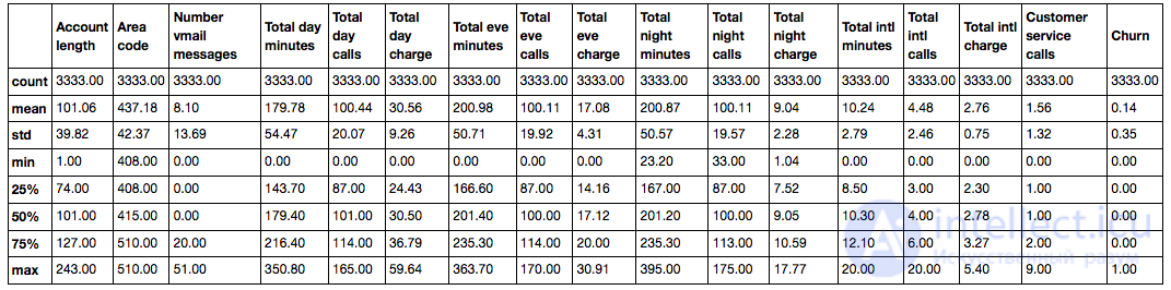
To see statistics for non-numeric features, we need to explicitly specify the types we're interested in via the include parameter.

df.describe(include=['object', 'bool'])

For categorical (type object) and boolean (type bool) features, you can use the value_counts method. Let's look at the distribution of values for our target variable — Churn:

df['Churn'].value_counts()

0    2850
1     483
Name: Churn, dtype: int64

2850 out of 3333 users — are loyal, the value of the Churn variable for them — is 0.

Let's look at the distribution of users by the Area code variable. We'll set the normalize=True parameter to see relative frequencies instead of absolute ones.

df['Area code'].value_counts(normalize=True)

415    0.496550
510    0.252025
408    0.251425
Name: Area code, dtype: float64

Sorting

A DataFrame can be sorted by the value of one of the features. In our case, for example, by Total day charge (ascending=False for descending order):

df.sort_values(by='Total day charge', 
        ascending=False).head()

You can also sort by a group of columns:

df.sort_values(by=['Churn', 'Total day charge'],
        ascending=[True, False]).head()

thanks for the note about the outdated sort makkos

Indexing and Retrieving Data

A DataFrame can be indexed in different ways. With this in mind, let's look at various methods of indexing and retrieving the data we need from a dataframe using simple questions as examples.

To retrieve a single column, you can use a construct like DataFrame['Name']. Let's use this to answer the question: what is the share of disloyal users in our dataframe?

df['Churn'].mean(). # outputs: 0.14491449144914492

14,5% — a rather poor figure for a company; with such a churn rate, you could even go bankrupt.

Boolean indexing of a DataFrame by a single column is very convenient. It looks like this: df[P(df['Name'])], where P — is some boolean condition checked for each element of the Name column. The result of such indexing is a DataFrame consisting only of the rows that satisfy condition P on the Name column.

Let's use this to answer the question: what are the average values of the numeric features among disloyal users?

df[df['Churn'] == 1].mean()

Account length            102.664596
Number vmail messages       5.115942
Total day minutes         206.914079
Total day calls           101.335404
Total day charge           35.175921
Total eve minutes         212.410145
Total eve calls           100.561077
Total eve charge           18.054969
Total night minutes       205.231677
Total night calls         100.399586
Total night charge          9.235528
Total intl minutes         10.700000
Total intl calls            4.163561
Total intl charge           2.889545
Customer service calls      2.229814
Churn                       1.000000
dtype: float64

By combining the previous two types of indexing, let's answer the question: on average, how long do disloyal users talk on the phone during the day?

df[df['Churn'] == 1]['Total day minutes'].mean() # outputs: 206.91407867494823

What is the maximum length of international calls among loyal users (Churn == 0) who do not use the international roaming service ('International plan' == 'No')?

df[(df['Churn'] == 0) & (df['International plan'] == 'No')]['Total intl minutes'].max() # outputs: 18.899999999999999

Dataframes can be indexed either by the name of a column or row, or by their ordinal position. The loc method is used for indexing by name, and iloc — for indexing by position.

In the first case, we're saying «give us the values for rows with id from 0 to 5 and for columns from State to Area code», and in the second — «give us the values of the first five rows in the first three columns».

Note to self: when we pass a slice object to iloc, the dataframe is sliced as usual. However, in the case of loc, both the start and the end of the slice are taken into account (link to the documentation, thanks to arkane0906 for the note).

df.loc[0:5, 'State':'Area code']

df.iloc[0:5, 0:3]

If we need the first or last row of the dataframe, we use the construct df[:1] or df[-1:]:

df[-1:]

Applying Functions to Cells, Columns, and Rows

Applying a function to each column: apply

df.apply(np.max) 

State                        WY
Account length              243
Area code                   510
International plan          Yes
Voice mail plan             Yes
Number vmail messages        51
Total day minutes         350.8
Total day calls             165
Total day charge          59.64
Total eve minutes         363.7
Total eve calls             170
Total eve charge          30.91
Total night minutes         395
Total night calls           175
Total night charge        17.77
Total intl minutes           20
Total intl calls             20
Total intl charge           5.4
Customer service calls        9
Churn                      True
dtype: object

The apply method can also be used to apply a function to each row. To do this, you need to specify axis=1.

Applying a function to each cell of a column: map

For example, the map method can be used to replace values in a column by passing it a dictionary of the form {old_value: new_value} as an argument:

d = {'No' : False, 'Yes' : True}
df['International plan'] = df['International plan'].map(d)
df.head()

You can carry out the same operation using the replace method:

df = df.replace({'Voice mail plan': d})
df.head()

Grouping Data

In general, grouping data in Pandas looks like this:

df.groupby(by=grouping_columns)[columns_to_show].function()

1. The groupby method is applied to the dataframe, which splits the data by grouping_columns – a feature or set of features.
2. We select the columns we need (columns_to_show).
3. A function or several functions are applied to the resulting groups.

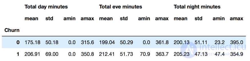
Grouping data based on the value of the Churn feature and displaying statistics for three columns within each group.

columns_to_show = ['Total day minutes', 'Total eve minutes', 'Total night minutes']

df.groupby(['Churn'])[columns_to_show].describe(percentiles=[])

Let's do the same thing, but slightly differently, by passing a list of functions to agg:

columns_to_show = ['Total day minutes', 'Total eve minutes', 'Total night minutes']

df.groupby(['Churn'])[columns_to_show].agg([np.mean, np.std, np.min, np.max])

Pivot Tables

Suppose we want to see how the observations in our sample are distributed with respect to two features — Churn and International plan. To do this, we can build a contingency table using the crosstab method:

pd.crosstab(df['Churn'], df['International plan'])

pd.crosstab(df['Churn'], df['Voice mail plan'], normalize=True)

We see that most users are loyal and also use additional services (international roaming / voicemail).

Advanced Excel users will surely remember a feature called pivot tables. In Pandas, pivot tables are handled by the pivot_table method, which takes the following parameters:

• values – the list of variables for which we need to calculate the desired statistics,
• index – the list of variables by which the data should be grouped,
• aggfunc — what we actually need to calculate for the groups — the sum, mean, maximum, minimum, or something else.

Let's look at the average number of day, evening, and night calls for different Area codes:

df.pivot_table(['Total day calls', 'Total eve calls', 'Total night calls'], 
['Area code'], aggfunc='mean').head(10)

Transforming Dataframes

As with many other things in Pandas, adding columns to a DataFrame can be done in several ways.

For example, suppose we want to calculate the total number of calls for all users. Let's create a total_calls object of type Series and insert it into the dataframe:

total_calls = df['Total day calls'] + df['Total eve calls'] + \
                  df['Total night calls'] + df['Total intl calls']
df.insert(loc=len(df.columns), column='Total calls', value=total_calls) 
# loc - the column number after which to insert this Series
# we specified len(df.columns) to insert it at the very end
df.head()

Adding a column from existing ones can also be done more simply, without creating intermediate Series objects:

df['Total charge'] = df['Total day charge'] + df['Total eve charge'] + df['Total night charge'] + df['Total intl charge']

df.head()

To delete columns or rows, use the drop method, passing the needed indices as an argument along with the required value of the axis parameter (1 if you're deleting columns, and nothing or 0 if you're deleting rows):

# get rid of the columns we just created
df = df.drop(['Total charge', 'Total calls'], axis=1) 

df.drop([1, 2]).head() # and this is how you can delete rows

4. First Attempts at Predicting Churn

Let's look at how churn relates to the feature "International roaming enabled" (International plan). We'll do this using the crosstab pivot table, as well as by illustrating it with Seaborn (exactly how to build such plots and analyze them – that's material for the next article).

pd.crosstab(df['Churn'], df['International plan'], margins=True)

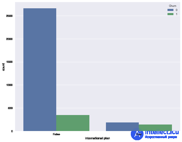
We see that when roaming is enabled, the churn rate is much higher – an interesting observation! Perhaps large and poorly controlled roaming expenses are a major source of friction and lead to customer dissatisfaction with the telecom operator, and consequently to churn.

Next, let's look at another important feature – "Number of calls to customer service" (Customer service calls). We'll also build a pivot table and a plot.

pd.crosstab(df['Churn'], df['Customer service calls'], margins=True)

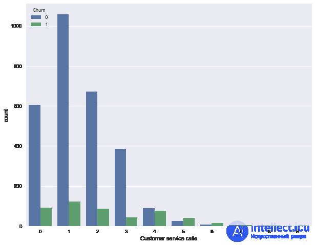
It may not be so easy to see from the pivot table alone (or it's tedious to scan through rows of numbers), but the plot clearly shows that the churn rate increases sharply starting from 4 calls to customer service.

Let's now add a binary feature to our DataFrame — the result of comparing Customer service calls > 3. And let's look once more at how it relates to churn.

df['Many_service_calls'] = (df['Customer service calls'] > 3).astype('int')

pd.crosstab(df['Many_service_calls'], df['Churn'], margins=True)

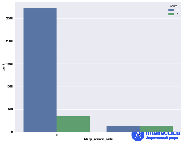
Let's combine the conditions considered above and build a pivot table for this combination and churn.

pd.crosstab(df['Many_service_calls'] & df['International plan'] , df['Churn'])

This means that by predicting customer churn when the number of calls to customer service is greater than 3 and roaming is enabled (and predicting loyalty – otherwise), we can expect around 85.8% correct hits (we're wrong only 464 + 9 times). This 85.8%, which we obtained using very simple reasoning – is a pretty good starting point (baseline) for the further machine learning models we will build.

In general, before the advent of machine learning, the data analysis process looked roughly like this. Let's summarize:

• The share of loyal customers in the sample – 85.5%. The most naive model, whose answer is "the customer is always loyal", will guess correctly about 85.5% of the time on data like this. That is, the share of correct answers (accuracy) of subsequent models should be at least no lower, and preferably significantly higher, than this figure;
• Using a simple prediction, which can be conditionally expressed by the formula: "International plan = True & Customer Service calls > 3 => Churn = 1, else Churn = 0", we can expect a guessing accuracy of 85.8%, which is a bit higher than 85.5%. Later we will talk about decision trees and figure out how to find such rules automatically based only on the input data;
• We obtained these two baselines without any machine learning, and they serve as a starting point for our subsequent models. If it turns out that with enormous effort we increase the share of correct answers by only, say, 0.5%, then perhaps we're doing something wrong, and it's enough to stick with a simple model based on two conditions;
• Before training complex models, it's recommended to poke around the data a bit and check simple assumptions. Moreover, in business applications of machine learning, people most often start with simple solutions and then experiment with making them more complex.

5. Homework Assignment #1

From now on, the course will be conducted in English (the articles are also available on Medium). The next run starts – October 1, 2018.

As a warm-up/preparation exercise, we suggest analyzing demographic data using Pandas. You need to fill in the missing code in the Jupyter template and choose the correct answers in the web form (you'll also find the solution there).

6. Overview of Useful Resources

• Translation of this article into English – Medium story
• Video recording of a lecture based on this article
• First and foremost, of course, the official Pandas documentation. In particular, we recommend the short introduction 10 minutes to pandas
• Russian translation of the book "Learning pandas" + repository
• PDF cheat sheet for the library
• Presentation by Alexander Dyakonov «Introduction to Pandas»
• The "Modern Pandas" series of posts (in English)
• On GitHub there's a collection of Pandas exercises and another useful repository (in English) "Effective Pandas"
• scipy-lectures.org — a tutorial on working with pandas, numpy, matplotlib, and scikit-learn
• Pandas From The Ground Up – video from PyCon 2015