
Lecture
Good day! We continue our series of articles for the open machine learning course, and today we'll talk about time series.
 Let's look at how to work with them in Python, what possible methods and models can be used for forecasting; what double and triple exponential smoothing are; what to do if stationarity isn't your thing; how to build a SARIMA and not die trying; and how to forecast with xgboost. And we'll apply all of this to an example from harsh reality.
UPD: the course is now available in English under the mlcourse.ai brand, with articles on Medium, and materials on Kaggle (Dataset) and on GitHub.
A video recording of the lecture based on this article, from the second run of the open course (September–November 2017).
List of articles in the series
Plan of this article:
At work, I deal with time series-related tasks almost every day. Most often the question comes up — what will happen to our metrics in the near day/week/month/etc. — how many players will install the app, how many will be online, how many actions users will perform, and so on. The forecasting problem can be approached in different ways, depending on what quality the forecast needs to be, what period we want to build it for, and, of course, how long we can spend selecting and tuning the model's parameters to obtain it.
Let's start with simple methods of analysis and forecasting — moving averages, smoothing, and their variations.
A brief definition of a time series:
A time series – is a sequence of values describing a process that unfolds over time, measured at successive points in time, usually at equal intervals
Thus, the data turns out to be ordered with respect to non-random points in time, and, therefore, unlike random samples, may contain additional information that we will try to extract.
Let's import the necessary libraries. Mainly we'll need the statsmodels module, which implements numerous statistical modeling methods, including for time series. For fans of R who switched to Python, it may feel very familiar, since it supports writing model formulas in the style of 'Wage ~ Age + Education'.
import sys
import warnings
warnings.filterwarnings('ignore')
from tqdm import tqdm

import pandas as pd
import numpy as np
from sklearn.metrics import mean_absolute_error, mean_squared_error

import statsmodels.formula.api as smf
import statsmodels.tsa.api as smt
import statsmodels.api as sm
import scipy.stats as scs
from scipy.optimize import minimize

import matplotlib.pyplot as plt
As a working example, we'll take real data on hourly online player counts in one of the mobile games:
Code for plotting the chart
from plotly.offline import download_plotlyjs, init_notebook_mode, plot, iplot
from plotly import graph_objs as go
init_notebook_mode(connected = True)

def plotly_df(df, title = ''):
    data = []

    for column in df.columns:
        trace = go.Scatter(
            x = df.index,
            y = df[column],
            mode = 'lines',
            name = column
        )
        data.append(trace)

    layout = dict(title = title)
    fig = dict(data = data, layout = layout)
    iplot(fig, show_link=False)

dataset = pd.read_csv('hour_online.csv', index_col=['Time'], parse_dates=['Time'])
plotly_df(dataset, title = "Online users")
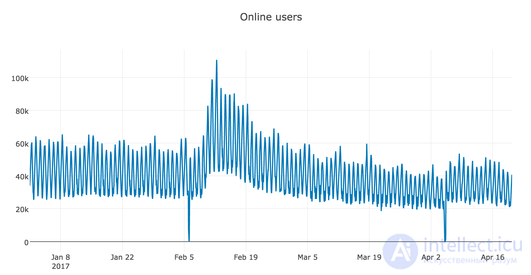
Let's start modeling with a naive assumption — "tomorrow will be like yesterday", but instead of a model of the form  we will assume that the future value of the variable depends on the average
  of its previous values, and thus we'll use the moving average.
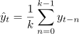
Let's implement the same function in Python and look at the forecast built from the last observed day (24 hours)
def moving_average(series, n):
    return np.average(series[-n:])

moving_average(dataset.Users, 24)
Out: 29858.333333333332
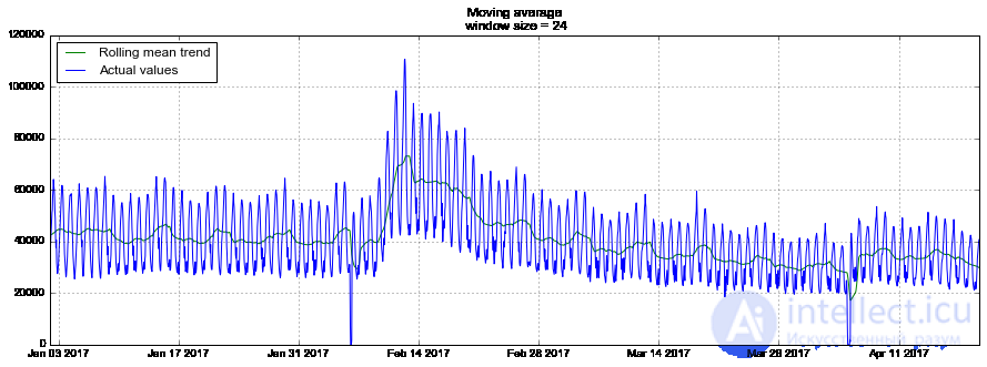
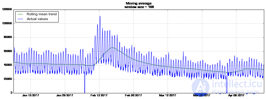
Unfortunately, it won't be possible to make such a forecast long-term — to get a one-step-ahead prediction, the previous value must actually be an observed quantity. On the other hand, the moving average has another use — smoothing the original series to reveal trends. Pandas has a ready-made implementation — DataFrame.rolling(window).mean(). The larger the interval width we set, the smoother the resulting trend will be. If the data is heavily noisy, which is especially common, for example, in financial indicators, such a procedure can help identify general patterns.
For our series, the trends are already quite obvious, but if we smooth by day, the dynamics of the online count on weekdays and weekends become more visible (weekends — time to play), and weekly smoothing nicely reflects the overall changes associated with the sharp rise in the number of active players in February and the subsequent decline in March.
Code for plotting the chart
def plotMovingAverage(series, n):

    """
    series - dataframe with timeseries
    n - rolling window size

    """

    rolling_mean = series.rolling(window=n).mean()

    # If desired, confidence intervals for the smoothed values can also be built
    #rolling_std =  series.rolling(window=n).std()
    #upper_bond = rolling_mean+1.96*rolling_std
    #lower_bond = rolling_mean-1.96*rolling_std

    plt.figure(figsize=(15,5))
    plt.title("Moving average\n window size = {}".format(n))
    plt.plot(rolling_mean, "g", label="Rolling mean trend")

    #plt.plot(upper_bond, "r--", label="Upper Bond / Lower Bond")
    #plt.plot(lower_bond, "r--")
    plt.plot(dataset[n:], label="Actual values")
    plt.legend(loc="upper left")
    plt.grid(True)
plotMovingAverage(dataset, 24) # smooth by day
plotMovingAverage(dataset, 24*7) # smooth by week
A modification of the simple moving average is the weighted average, in which observations are assigned different weights that sum to one, with the most recent observations usually given a larger weight.
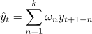
def weighted_average(series, weights):
    result = 0.0
    weights.reverse()
    for n in range(len(weights)):
        result += series[-n-1] * weights[n]
    return result

weighted_average(dataset.Users, [0.6, 0.2, 0.1, 0.07, 0.03])
Out: 35967.550000000003
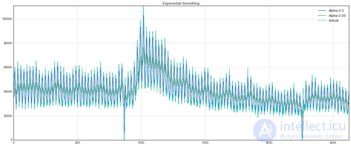
Now let's see what happens if, instead of weighting the last values of the series, we start weighting all available observations, exponentially decreasing the weights as we go deeper into the historical data. The formula for simple exponential smoothing will help us here:

Here the model value is a weighted average between the current true value and the previous model value. The weight  is called the smoothing factor. It determines how quickly we will "forget" the last available true observation. The smaller is, the greater the influence of previous model values, and the stronger the series is smoothed.
The exponential nature is hidden in the recursiveness of the function — each time we multiply  by the previous model value, which, in turn, also contained , and so on all the way back to the beginning.
def exponential_smoothing(series, alpha):
    result = [series[0]] # first value is same as series
    for n in range(1, len(series)):
        result.append(alpha * series[n] + (1 - alpha) * result[n-1])
    return result
Code for plotting the chart
with plt.style.context('seaborn-white'):
    plt.figure(figsize=(20, 8))
    for alpha in [0.3, 0.05]:
        plt.plot(exponential_smoothing(dataset.Users, alpha), label="Alpha {}".format(alpha))
    plt.plot(dataset.Users.values, "c", label = "Actual")
    plt.legend(loc="best")
    plt.axis('tight')
    plt.title("Exponential Smoothing")
    plt.grid(True)
So far, the best our methods could give us was a forecast just one point ahead (and also a nicely smoothed series), which is great, but not enough, so we move on to an extension of exponential smoothing that lets us build a forecast two points ahead at once (and also nicely smooth the series).
Splitting the series into two components will help us here — the level (level, intercept)  and the trend
  (trend, slope). We predicted the level, or the expected value of the series, using the previous methods, and now we'll apply the same exponential smoothing to the trend, naively or not so naively assuming that the future direction of the series' change depends on the weighted previous changes.

As a result we get a set of functions. The first describes the level — as before, it depends on the current value of the series, but the second term is now split into the previous value of the level and the trend. The second describes the trend — it depends on the change of the level at the current step, and on the previous value of the trend. Here, the role of weight in the exponential smoothing is played by the coefficient  . Finally, the final prediction is the sum of the model values of the level and the trend.
def double_exponential_smoothing(series, alpha, beta):
    result = [series[0]]
    for n in range(1, len(series)+1):
        if n == 1:
            level, trend = series[0], series[1] - series[0]
        if n >= len(series): # forecasting
            value = result[-1]
        else:
            value = series[n]
        last_level, level = level, alpha*value + (1-alpha)*(level+trend)
        trend = beta*(level-last_level) + (1-beta)*trend
        result.append(level+trend)
    return result
Code for plotting the chart
with plt.style.context('seaborn-white'):
    plt.figure(figsize=(20, 8))
    for alpha in [0.9, 0.02]:
        for beta in [0.9, 0.02]:
            plt.plot(double_exponential_smoothing(dataset.Users, alpha, beta), label="Alpha {}, beta {}".format(alpha, beta))
    plt.plot(dataset.Users.values, label = "Actual")
    plt.legend(loc="best")
    plt.axis('tight')
    plt.title("Double Exponential Smoothing")
    plt.grid(True)
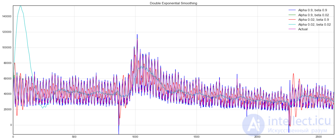
Now we already had two parameters to tune — and . The first is responsible for smoothing the series around the trend, the second — for smoothing the trend itself. The higher the values, the greater the weight given to the most recent observations, and the less smoothed the model series will turn out. Combinations of parameters can produce quite whimsical results, especially if you set them by hand. I'll talk about non-manual parameter tuning a bit further below, right after triple exponential smoothing.
So, we've successfully made it to the next variant of exponential smoothing, this time the triple one.
The idea of this method is to add one more, third, component — seasonality. Accordingly, the method is applicable only if the series is not devoid of this seasonality, which is true in our case. The seasonal component in the model will explain the repeating fluctuations around the level and the trend, and it will be characterized by the season length — the period after which the fluctuations start repeating. A separate component is formed for each observation in the season, for example, if the season length is 7 (e.g., weekly seasonality), then we get 7 seasonal components, one for each day of the week.
We get a new system:

The level now depends on the current value of the series minus the corresponding seasonal component, the trend remains unchanged, and the seasonal component depends on the current value of the series minus the level and on the previous value of the component. Here, the components are smoothed across all available seasons, for example, if this is the component responsible for Monday, then it will only be averaged with other Mondays. You can read more about how the averaging works and how the initial values of the trend and seasonal components are estimated here. Now, having the seasonal component, we can forecast not just one, or even two, but an arbitrary  steps ahead, which is certainly a nice thing.
Below is the code for building the triple exponential smoothing model, also known by the names of its creators — Charles Holt and his student Peter Winters.
Additionally, the Brutlag method for building confidence intervals is included in the model:
$$display$$ \hat y_{max_x}=\ell_{x−1}+b_{x−1}+s_{x−T}+m⋅d_{t−T}\\ \hat y_{min_x}=\ell_{x−1}+b_{x−1}+s_{x−T}-m⋅d_{t−T}\\ d_t=\gamma∣y_t−\hat y_t∣+(1−\gamma)d_{t−T}, $$display$$
where  — the season length,
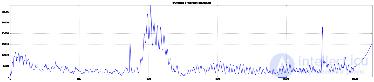
  — the predicted deviation, and the remaining parameters are taken from the triple smoothing. You can read more about the method and its application to anomaly detection in time series here
Code for the Holt-Winters model
class HoltWinters:

    """
    Holt-Winters model with the Brutlag method for anomaly detection
    https://fedcsis.org/proceedings/2012/pliks/118.pdf

    # series - the original time series
    # slen - the season length
    # alpha, beta, gamma - the coefficients of the Holt-Winters model
    # n_preds - the forecast horizon
    # scaling_factor - sets the width of the Brutlag confidence interval (usually takes values from 2 to 3)

    """

    def __init__(self, series, slen, alpha, beta, gamma, n_preds, scaling_factor=1.96):
        self.series = series
        self.slen = slen
        self.alpha = alpha
        self.beta = beta
        self.gamma = gamma
        self.n_preds = n_preds
        self.scaling_factor = scaling_factor

    def initial_trend(self):
        sum = 0.0
        for i in range(self.slen):
            sum += float(self.series[i+self.slen] - self.series[i]) / self.slen
        return sum / self.slen

    def initial_seasonal_components(self):
        seasonals = {}
        season_averages = []
        n_seasons = int(len(self.series)/self.slen)
        # calculate the seasonal averages
        for j in range(n_seasons):
            season_averages.append(sum(self.series[self.slen*j:self.slen*j+self.slen])/float(self.slen))
        # calculate the initial values
        for i in range(self.slen):
            sum_of_vals_over_avg = 0.0
            for j in range(n_seasons):
                sum_of_vals_over_avg += self.series[self.slen*j+i]-season_averages[j]
            seasonals[i] = sum_of_vals_over_avg/n_seasons
        return seasonals

    def triple_exponential_smoothing(self):
        self.result = []
        self.Smooth = []
        self.Season = []
        self.Trend = []
        self.PredictedDeviation = []
        self.UpperBond = []
        self.LowerBond = []

        seasonals = self.initial_seasonal_components()

        for i in range(len(self.series)+self.n_preds):
            if i == 0: # initialize the component values
                smooth = self.series[0]
                trend = self.initial_trend()
                self.result.append(self.series[0])
                self.Smooth.append(smooth)
                self.Trend.append(trend)
                self.Season.append(seasonals[i%self.slen])

                self.PredictedDeviation.append(0)

                self.UpperBond.append(self.result[0] +
                                      self.scaling_factor *
                                      self.PredictedDeviation[0])

                self.LowerBond.append(self.result[0] -
                                      self.scaling_factor *
                                      self.PredictedDeviation[0])

                continue
            if i >= len(self.series): # forecasting
                m = i - len(self.series) + 1
                self.result.append((smooth + m*trend) + seasonals[i%self.slen])

                # during forecasting, increase the uncertainty with each step
                self.PredictedDeviation.append(self.PredictedDeviation[-1]*1.01)

            else:
                val = self.series[i]
                last_smooth, smooth = smooth, self.alpha*(val-seasonals[i%self.slen]) + (1-self.alpha)*(smooth+trend)
                trend = self.beta * (smooth-last_smooth) + (1-self.beta)*trend
                seasonals[i%self.slen] = self.gamma*(val-smooth) + (1-self.gamma)*seasonals[i%self.slen]
                self.result.append(smooth+trend+seasonals[i%self.slen])

                # the deviation is calculated according to the Brutlag algorithm
                self.PredictedDeviation.append(self.gamma * np.abs(self.series[i] - self.result[i])
                                               + (1-self.gamma)*self.PredictedDeviation[-1])

            self.UpperBond.append(self.result[-1] +
                                  self.scaling_factor *
                                  self.PredictedDeviation[-1])

            self.LowerBond.append(self.result[-1] -
                                  self.scaling_factor *
                                  self.PredictedDeviation[-1])

            self.Smooth.append(smooth)
            self.Trend.append(trend)
            self.Season.append(seasonals[i % self.slen])
Before building the model, let's finally talk about non-manual estimation of parameters for the models.
There's nothing unusual here, as before we first need to choose a loss function suitable for the given task: RMSE, MAE, MAPE, etc., which will monitor the quality of the model's fit to the source data. Then we'll estimate the value of the loss function for given model parameters using cross-validation, look for the gradient, adjust the parameters accordingly, and briskly descend towards the global minimum of the error.
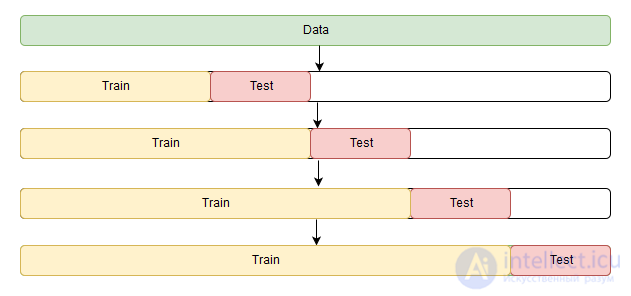
A small snag arises only in cross-validation. The problem is that a time series, paradoxically, has a temporal structure, and it's not possible to randomly shuffle the values of the whole series across folds without preserving this structure, otherwise all the relationships between observations would be lost in the process. So we'll have to use a slightly trickier way to optimize the parameters, for which I haven't found an official name, but on the CrossValidated site, where you can find answers to everything except the main question of Life, the Universe, and Everything, they suggest the name "cross-validation on a rolling basis", which can be loosely translated as cross-validation on a sliding window.
The idea is quite simple — we start training the model on a small segment of the time series, from the beginning to some  , make a forecast
  steps ahead and calculate the error. Next we extend the training set to the value and forecast from to
  , and continue moving the test segment of the series like this until we hit the last available observation. In the end we get as many folds as fit into the gap between the initial training segment and the full length of the series.
Code for cross-validation on a time series
from sklearn.model_selection import TimeSeriesSplit

def timeseriesCVscore(x):
    # vector of errors
    errors = []

    values = data.values
    alpha, beta, gamma = x

    # set the number of folds for cross-validation
    tscv = TimeSeriesSplit(n_splits=3)

    # go through the folds, train the model on each, build a forecast on the held-out sample and calculate the error
    for train, test in tscv.split(values):

        model = HoltWinters(series=values[train], slen = 24*7, alpha=alpha, beta=beta, gamma=gamma, n_preds=len(test))
        model.triple_exponential_smoothing()

        predictions = model.result[-len(test):]
        actual = values[test]
        error = mean_squared_error(predictions, actual)
        errors.append(error)

    # Return the mean squared error over the vector of errors
    return np.mean(np.array(errors))
The season length value of 24*7 didn't come about by chance — the original series clearly shows daily seasonality (hence the 24), and weekly seasonality — lower on weekdays, higher on weekends (hence the 7), giving a total of 24*7 seasonal components.
In the Holt-Winters model, as in other exponential smoothing models, there's a constraint on the value of the smoothing parameters — each of them can take values from 0 to 1, so to minimize the loss function we need to choose an algorithm that supports constraints on the parameters, in this case — Truncated Newton conjugate gradient.
%%time
data = dataset.Users[:-500] # set aside part of the data for testing

# initialize the parameter values
x = [0, 0, 0]

# Minimize the loss function with constraints on the parameters
opt = minimize(timeseriesCVscore, x0=x, method="TNC", bounds = ((0, 1), (0, 1), (0, 1)))

# Take the optimal parameter values from the optimizer
alpha_final, beta_final, gamma_final = opt.x
print(alpha_final, beta_final, gamma_final)
Out: (0.0066342670643441681, 0.0, 0.046765204289672901)
Let's pass the obtained optimal coefficient values , and  and build a forecast 5 days ahead (128 hours)
# Pass the optimal values to the model,
data = dataset.Users
model = HoltWinters(data[:-128], slen = 24*7, alpha = alpha_final, beta = beta_final, gamma = gamma_final, n_preds = 128, scaling_factor = 2.56)
model.triple_exponential_smoothing()
Code for plotting the chart
def plotHoltWinters():
    Anomalies = np.array([np.NaN]*len(data))
    Anomalies[data.values
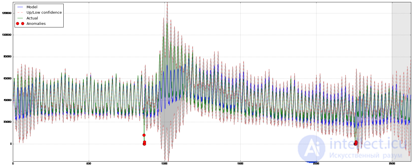
Judging by the chart, the model described the original time series quite well, capturing the weekly and daily seasonality, and even managed to catch anomalous drops that went beyond the confidence intervals. If we look at the modeled deviation, we can clearly see that the model reacts fairly sharply to significant changes in the structure of the series, but at the same time quickly returns the variance to normal values, "forgetting" the past. This feature makes it possible to set up an anomaly detection system quite well, without significant costs for preparing and training the model, even on fairly noisy series.
Before moving on to modeling, it's worth mentioning such an important property of a time series as stationarity. Stationarity is understood as the property of a process not to change its statistical characteristics over time, namely constancy of the expected value, constancy of variance (also known as homoscedasticity), and independence of the covariance function from time (it should depend only on the distance between observations). These properties can be seen clearly in the pictures taken from Sean Abu's post:
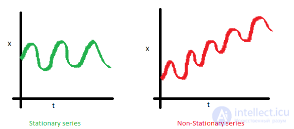
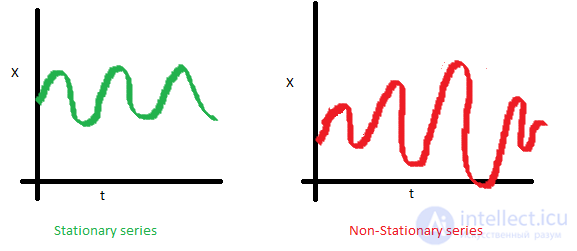
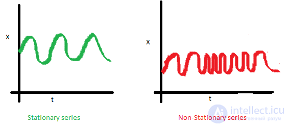
Why is stationarity so important? A stationary series is easy to forecast, since we assume that its future statistical characteristics will not differ from the currently observed ones. Most time series models, in one way or another, model and predict these characteristics (for example, the expected value or the variance), so in the case of non-stationarity of the original series, the predictions will turn out to be wrong. Unfortunately, most of the time series one has to deal with outside of educational materials are not stationary, but this can (and should) be dealt with.
To fight non-stationarity, we need to know it by sight, so let's look at how to detect it. To do this, we'll turn to white noise and a random walk, to figure out how to get from one to the other for free and without any hassle.
A plot of white noise:
white_noise = np.random.normal(size=1000)
with plt.style.context('bmh'):
    plt.figure(figsize=(15, 5))
    plt.plot(white_noise)
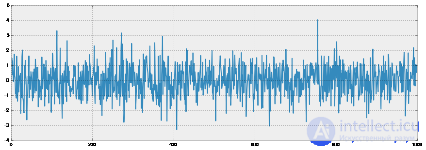
So, a process generated by a standard normal distribution is stationary, fluctuating around zero with a deviation of 1. Now, based on it, let's generate a new process in which each subsequent value depends on the previous one: 
Code for plotting the graphs
def plotProcess(n_samples=1000, rho=0):
    x = w = np.random.normal(size=n_samples)
    for t in range(n_samples):
        x[t] = rho * x[t-1] + w[t]

    with plt.style.context('bmh'):
        plt.figure(figsize=(10, 3))
        plt.plot(x)
        plt.title("Rho {}\n Dickey-Fuller p-value: {}".format(rho, round(sm.tsa.stattools.adfuller(x)[1], 3)))

for rho in [0, 0.6, 0.9, 1]:
    plotProcess(rho=rho)
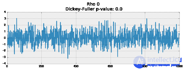
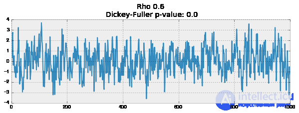
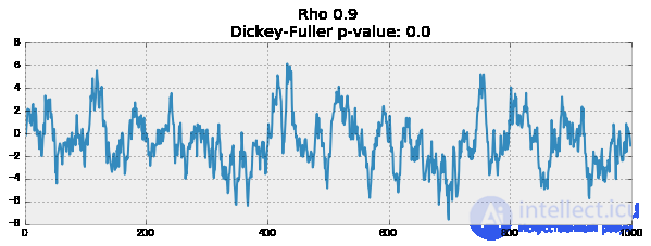
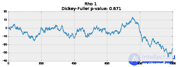
The first plot turned out to be exactly the same stationary white noise that was built earlier. In the second one, the value of  increased to 0.6, as a result of which wider cycles began to appear in the plot, but overall it hasn't stopped being stationary yet. The third plot deviates more and more strongly from a zero mean, but still fluctuates around it. Finally, the value of equal to one produced a random walk process — the series is not stationary.
This happens because once the critical value of one is reached, the series stops returning to its mean value. If we subtract  from the left and right sides, we get
  , where the expression on the left is the first differences. If
  , then the first differences will give stationary white noise
  . This fact forms the basis of the Dickey-Fuller test for stationarity of a series (the presence of a unit root). If a stationary series can be obtained from a non-stationary one by first differencing, it is called integrated of order one. The null hypothesis of the test — that the series is not stationary — was rejected for the first three plots, and accepted for the last one. It's worth saying that first differences are not always enough to obtain a stationary series, since the process may be integrated of a higher order (have several unit roots); to check such cases, the augmented Dickey-Fuller test is used, which checks several lags at once.
Non-stationarity can be dealt with in many ways — differencing of various orders, extracting the trend and seasonality, smoothing, and transformations such as Box-Cox or taking the logarithm.
Let's now try to build an ARIMA model for the number of online players, going through all the circles of hell of the stage of bringing the series to a stationary form. You can read about the model itself in other articles of this section — Building a SARIMA model with Python+R, Time series analysis with python, so I won't dwell on it in detail.
Code for plotting the graphs
def tsplot(y, lags=None, figsize=(12, 7), style='bmh'):
    if not isinstance(y, pd.Series):
        y = pd.Series(y)
    with plt.style.context(style):
        fig = plt.figure(figsize=figsize)
        layout = (2, 2)
        ts_ax = plt.subplot2grid(layout, (0, 0), colspan=2)
        acf_ax = plt.subplot2grid(layout, (1, 0))
        pacf_ax = plt.subplot2grid(layout, (1, 1))

        y.plot(ax=ts_ax)
        ts_ax.set_title('Time Series Analysis Plots')
        smt.graphics.plot_acf(y, lags=lags, ax=acf_ax, alpha=0.5)
        smt.graphics.plot_pacf(y, lags=lags, ax=pacf_ax, alpha=0.5)

        print("Dickey-Fuller criterion: p=%f" % sm.tsa.stattools.adfuller(y)[1])

        plt.tight_layout()
    return

tsplot(dataset.Users, lags=30)
Out: Dickey-Fuller criterion: p=0.190189
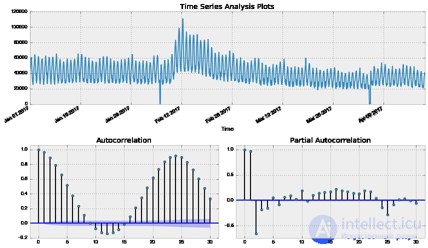
As expected, the original series is not stationary; the Dickey-Fuller criterion did not reject the null hypothesis of the presence of a unit root. Let's try to stabilize the variance with a Box-Cox transformation.
def invboxcox(y,lmbda):
    # inverse Box-Cox transformation
    if lmbda == 0:
        return(np.exp(y))
    else:
        return(np.exp(np.log(lmbda*y+1)/lmbda))

data = dataset.copy()
data['Users_box'], lmbda = scs.boxcox(data.Users+1) # add one, since there are zeros in the original series
tsplot(data.Users_box, lags=30)
print("Optimal Box-Cox transformation parameter: %f" % lmbda)
Out: Dickey-Fuller criterion: p=0.079760
     Optimal Box-Cox transformation parameter: 0.587270
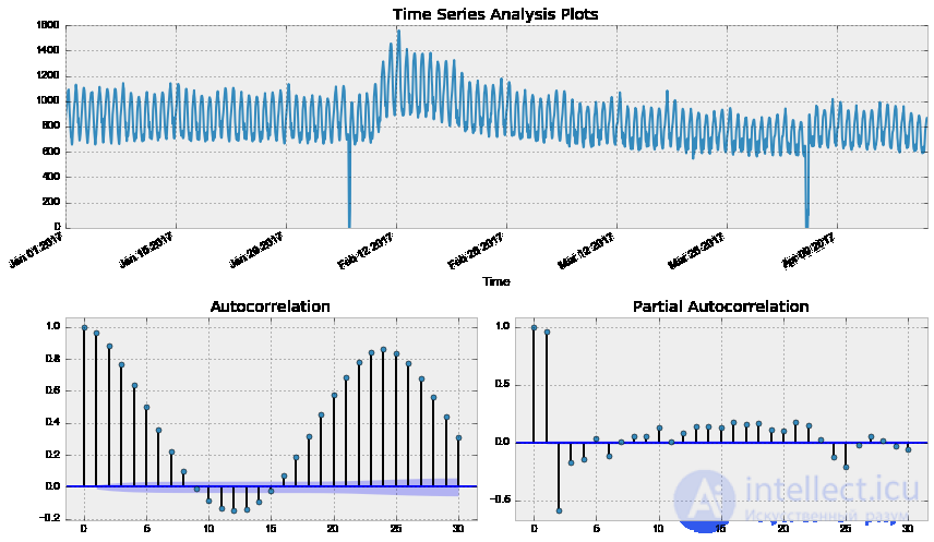
Already better, but the Dickey-Fuller criterion still does not reject the hypothesis of non-stationarity of the series. And the autocorrelation function clearly hints at seasonality in the resulting series. Let's take seasonal differences:
data['Users_box_season'] = data.Users_box - data.Users_box.shift(24*7)
tsplot(data.Users_box_season[24*7:], lags=30)
Out: Dickey-Fuller criterion: p=0.002571
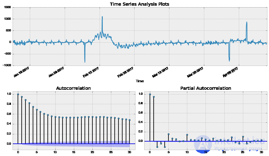
The Dickey-Fuller criterion now rejects the null hypothesis of non-stationarity, but the autocorrelation function still looks bad due to a large number of significant lags. Since only one lag is significant on the partial autocorrelation function plot, we should also take first differences to finally bring the series to a stationary form.
data['Users_box_season_diff'] = data.Users_box_season - data.Users_box_season.shift(1)
tsplot(data.Users_box_season_diff[24*7+1:], lags=30)
Out: Dickey-Fuller criterion: p=0.000000
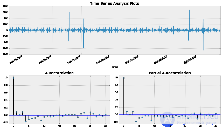
We have finally obtained a stationary series; based on the autocorrelation and partial autocorrelation functions, let's estimate the parameters for the SARIMA model, not forgetting that we have already made first and seasonal differences beforehand.
Initial approximations Q = 1, P = 4, q = 3, p = 4
ps = range(0, 5)
d=1
qs = range(0, 4)
Ps = range(0, 5)
D=1
Qs = range(0, 1)

from itertools import product

parameters = product(ps, qs, Ps, Qs)
parameters_list = list(parameters)
len(parameters_list)
Out: 100
Code for tuning parameters by grid search
%%time
results = []
best_aic = float("inf")

for param in tqdm(parameters_list):
    #try except is needed because the model fails to train on some parameter sets
    try:
        model=sm.tsa.statespace.SARIMAX(data.Users_box, order=(param[0], d, param[1]),
                                        seasonal_order=(param[2], D, param[3], 24*7)).fit(disp=-1)
    #print the parameters on which the model fails to train and move on to the next set
    except ValueError:
        print('wrong parameters:', param)
        continue
    aic = model.aic
    #save the best model, aic, parameters
    if aic < best_aic:
        best_model = model
        best_aic = aic
        best_param = param
    results.append([param, model.aic])

warnings.filterwarnings('default')

result_table = pd.DataFrame(results)
result_table.columns = ['parameters', 'aic']
print(result_table.sort_values(by = 'aic', ascending=True).head())
Let's plug the best parameters into the model:
%%time
best_model = sm.tsa.statespace.SARIMAX(data.Users_box, order=(4, d, 3),
                                        seasonal_order=(4, D, 1, 24)).fit(disp=-1)
print(best_model.summary())
                                 Statespace Model Results
==========================================================================================
Dep. Variable:                          Users_box   No. Observations:                 2625
Model:             SARIMAX(4, 1, 3)x(4, 1, 1, 24)   Log Likelihood              -12547.157
Date:                            Sun, 23 Apr 2017   AIC                          25120.315
Time:                                    02:06:39   BIC                          25196.662
Sample:                                         0   HQIC                         25147.964
                                           - 2625
Covariance Type:                              opg
==============================================================================
                 coef    std err          z      P>|z|      [0.025      0.975]
------------------------------------------------------------------------------
ar.L1          0.6794      0.108      6.310      0.000       0.468       0.890
ar.L2         -0.0810      0.181     -0.448      0.654      -0.435       0.273
ar.L3          0.3255      0.137      2.371      0.018       0.056       0.595
ar.L4         -0.2154      0.028     -7.693      0.000      -0.270      -0.161
ma.L1         -0.5086      0.106     -4.784      0.000      -0.717      -0.300
ma.L2         -0.0673      0.170     -0.395      0.693      -0.401       0.267
ma.L3         -0.3490      0.117     -2.976      0.003      -0.579      -0.119
ar.S.L24       0.1023      0.012      8.377      0.000       0.078       0.126
ar.S.L48      -0.0686      0.021     -3.219      0.001      -0.110      -0.027
ar.S.L72       0.1971      0.009     21.573      0.000       0.179       0.215
ar.S.L96      -0.1217      0.013     -9.279      0.000      -0.147      -0.096
ma.S.L24      -0.9983      0.045    -22.085      0.000      -1.087      -0.910
sigma2       873.4159     36.206     24.124      0.000     802.454     944.378
===================================================================================
Ljung-Box (Q):                      130.47   Jarque-Bera (JB):           1194707.99
Prob(Q):                              0.00   Prob(JB):                         0.00
Heteroskedasticity (H):               1.40   Skew:                             2.65
Prob(H) (two-sided):                  0.00   Kurtosis:                       107.88
===================================================================================

Warnings:
[1] Covariance matrix calculated using the outer product of gradients (complex-step).
Let's check the model's residuals:
tsplot(best_model.resid[24:], lags=30)
Out: Dickey-Fuller criterion: p=0.000000
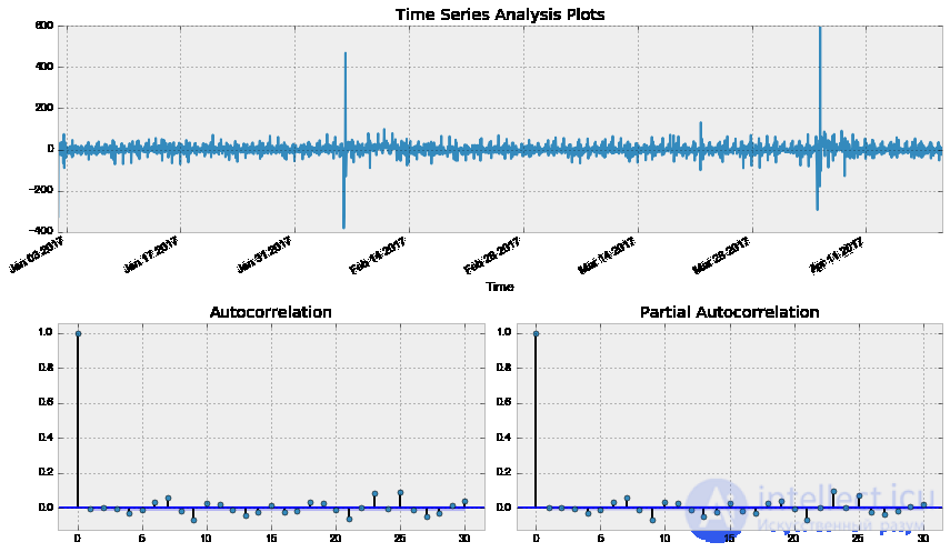
Well, the residuals are stationary, there are no obvious autocorrelations, let's build a forecast using the resulting model
Code for building the forecast and plotting the graph
data["arima_model"] = invboxcox(best_model.fittedvalues, lmbda)
forecast = invboxcox(best_model.predict(start = data.shape[0], end = data.shape[0]+100), lmbda)
forecast = data.arima_model.append(forecast).values[-500:]
actual = data.Users.values[-400:]
plt.figure(figsize=(15, 7))
plt.plot(forecast, color='r', label="model")
plt.title("SARIMA model\n Mean absolute error {} users".format(round(mean_absolute_error(data.dropna().Users, data.dropna().arima_model))))
plt.plot(actual, label="actual")
plt.legend()
plt.axvspan(len(actual), len(forecast), alpha=0.5, color='lightgrey')
plt.grid(True)
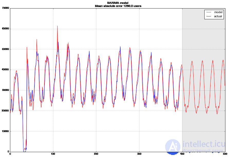
In the end we get a fairly adequate forecast; on average the model was off by 1.3K users, which is very, very good, however the total cost of data preparation, bringing the series to stationarity, and determining and searching through the parameters may not be worth this level of accuracy.
Once again, a small lyrical digression. At work you often have to build models guided by one fundamental principle – fast, good, cheap. Because of this, some models simply don't fit "production solutions", since they either require too much effort in data preparation (for example, SARIMA), or are hard to tune (a good example – SARIMA again), or require frequent retraining on new data (SARIMA again), so it's often much simpler to extract a few features from the available time series and build an ordinary linear regression on them, or slap a random forest on top. Cheap and cheerful.
This approach may not be strongly backed by theory and may violate various assumptions, for example the Gauss-Markov conditions, especially the point about the errors being uncorrelated, however in practice it often saves the day and is quite actively used in machine learning competitions.
Besides standard features like lags of the target variable, the date and time contain a lot of information. Extracting features from them has already been described nicely in one of the previous articles of the course.
I'll just add a note about one more way to encode categorical features – mean encoding. If you don't want to bloat the dataset with a bunch of dummy variables, which can lead to a loss of distance information, while in numeric form you get contradictory results along the lines of "0 hours < 23 hours", you can encode the variable with slightly more interpretable values. A natural option – encode it with the mean value of the target variable. In our case, each day of the week or hour of the day can be encoded with the corresponding average number of players who were online at that day of the week or hour. It's important to make sure that the mean is computed only within the training dataset (or within the current observed fold during cross-validation), otherwise you might accidentally leak information about the future into the model.
def code_mean(data, cat_feature, real_feature):
    """
    Returns a dictionary where the keys are unique categories of the cat_feature feature,
    and the values are means over real_feature
    """
    return dict(data.groupby(cat_feature)[real_feature].mean())
Let's create a new dataframe and add the hour, day of the week, and weekend flag as categorical variables. To do this, we convert the index that already exists in the dataframe to datetime format, and extract hour and weekday from it.
data = pd.DataFrame(dataset)
data.columns = ["y"]

data.index = data.index.to_datetime()
data["hour"] = data.index.hour
data["weekday"] = data.index.weekday
data['is_weekend'] = data.weekday.isin([5,6])*1
data.head()
Out:
| y | hour | weekday | is_weekend | |
|---|---|---|---|---|
| Time | ||||
| 2017-01-01 00:00:00 | 34002 | 0 | 6 | 1 |
| 2017-01-01 01:00:00 | 37947 | 1 | 6 | 1 |
| 2017-01-01 02:00:00 | 41517 | 2 | 6 | 1 |
| 2017-01-01 03:00:00 | 44476 | 3 | 6 | 1 |
| 2017-01-01 04:00:00 | 46234 | 4 | 6 | 1 |
Let's look at the averages by day of week
code_mean(data, 'weekday', "y")
Out:
{0: 38730.143229166664,
 1: 38632.828125,
 2: 38128.518229166664,
 3: 39519.035135135135,
 4: 41505.152777777781,
 5: 43717.708333333336,
 6: 43392.143603133161}
In addition to the transformations listed above, many other metrics are used to increase the number of features, for example, the maximum/minimum value observed in a sliding window over the series, medians, number of peaks, weighted variances, and much more. This is handled automatically by the tsfresh library already mentioned in the course.
For convenience, all the transformations can be written into a single function that will immediately return the datasets split into train and test, along with the target variables.
Function for creating variables
def prepareData(data, lag_start=5, lag_end=20, test_size=0.15):

    data = pd.DataFrame(data.copy())
    data.columns = ["y"]

    # calculate the index in the dataframe after which the test segment begins
    test_index = int(len(data)*(1-test_size))

    # add lags of the source series as features
    for i in range(lag_start, lag_end):
        data["lag_{}".format(i)] = data.y.shift(i)

    data.index = data.index.to_datetime()
    data["hour"] = data.index.hour
    data["weekday"] = data.index.weekday
    data['is_weekend'] = data.weekday.isin([5,6])*1

    # calculate averages only on the training part, to avoid a leak
    data['weekday_average'] = map(code_mean(data[:test_index], 'weekday', "y").get, data.weekday)
    data["hour_average"] = map(code_mean(data[:test_index], 'hour', "y").get, data.hour)

    # drop the features encoded by averages
    data.drop(["hour", "weekday"], axis=1, inplace=True)

    data = data.dropna()
    data = data.reset_index(drop=True)

    # split the whole dataset into training and test sets
    X_train = data.loc[:test_index].drop(["y"], axis=1)
    y_train = data.loc[:test_index]["y"]
    X_test = data.loc[test_index:].drop(["y"], axis=1)
    y_test = data.loc[test_index:]["y"]

    return X_train, X_test, y_train, y_test
Let's train a simple linear regression on the resulting data. In this case we will take lags starting from the twelfth, so the model will be able to build predictions 12 hours ahead, having actual observations for the previous half day.
Building a linear regression
from sklearn.linear_model import LinearRegression

X_train, X_test, y_train, y_test = prepareData(dataset.Users, test_size=0.3, lag_start=12, lag_end=48)
lr = LinearRegression()
lr.fit(X_train, y_train)
prediction = lr.predict(X_test)
plt.figure(figsize=(15, 7))
plt.plot(prediction, "r", label="prediction")
plt.plot(y_test.values, label="actual")
plt.legend(loc="best")
plt.title("Linear regression\n Mean absolute error {} users".format(round(mean_absolute_error(prediction, y_test))))
plt.grid(True);
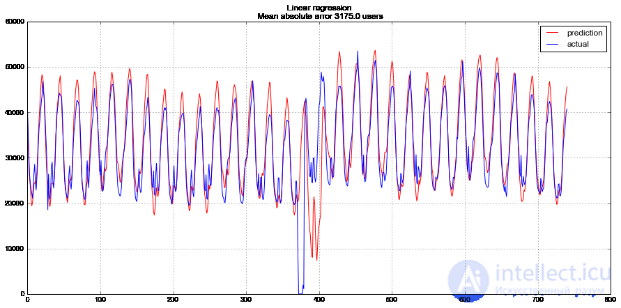
Got a fairly good result, even without feature selection the model is off, on average, by 3K users per hour, and this takes into account the huge outlier in the middle of the test series.
The model can also be evaluated using cross-validation, based on the same principle used earlier. For this we will use a function (with minor modifications) proposed in the post Pythonic Cross Validation on Time Series
Code for cross-validation
def performTimeSeriesCV(X_train, y_train, number_folds, model, metrics):
    print('Size train set: {}'.format(X_train.shape))

    k = int(np.floor(float(X_train.shape[0]) / number_folds))
    print('Size of each fold: {}'.format(k))

    errors = np.zeros(number_folds-1)

    # loop from the first 2 folds to the total number of folds
    for i in range(2, number_folds + 1):
        print('')
        split = float(i-1)/i
        print('Splitting the first ' + str(i) + ' chunks at ' + str(i-1) + '/' + str(i) )

        X = X_train[:(k*i)]
        y = y_train[:(k*i)]
        print('Size of train + test: {}'.format(X.shape)) # the size of the dataframe is going to be k*i

        index = int(np.floor(X.shape[0] * split))

        # folds used to train the model
        X_trainFolds = X[:index]
        y_trainFolds = y[:index]

        # fold used to test the model
        X_testFold = X[(index + 1):]
        y_testFold = y[(index + 1):]

        model.fit(X_trainFolds, y_trainFolds)
        errors[i-2] = metrics(model.predict(X_testFold), y_testFold)

    # the function returns the mean of the errors on the n-1 folds
    return errors.mean()
%%time
performTimeSeriesCV(X_train, y_train, 5, lr, mean_absolute_error)
Size train set: (1838, 39)
Size of each fold: 367

Splitting the first 2 chunks at 1/2
Size of train + test: (734, 39)

Splitting the first 3 chunks at 2/3
Size of train + test: (1101, 39)

Splitting the first 4 chunks at 3/4
Size of train + test: (1468, 39)

Splitting the first 5 chunks at 4/5
Size of train + test: (1835, 39)
CPU times: user 59.5 ms, sys: 7.02 ms, total: 66.5 ms
Wall time: 18.9 ms

Out: 4613.17893150896
On 5 folds we got a mean absolute error of 4.6 K users, fairly close to the quality estimate obtained on the test dataset.
Why not try XGBoost now...

Code for building a forecast with XGBoost
import xgboost as xgb

def XGB_forecast(data, lag_start=5, lag_end=20, test_size=0.15, scale=1.96):

    # source data
    X_train, X_test, y_train, y_test = prepareData(dataset.Users, lag_start, lag_end, test_size)
    dtrain = xgb.DMatrix(X_train, label=y_train)
    dtest = xgb.DMatrix(X_test)

    # set the parameters
    params = {
        'objective': 'reg:linear',
        'booster':'gblinear'
    }
    trees = 1000

    # run cross-validation with the rmse metric
    cv = xgb.cv(params, dtrain, metrics = ('rmse'), verbose_eval=False, nfold=10, show_stdv=False, num_boost_round=trees)

    # train xgboost with the optimal number of trees, selected via cross-validation
    bst = xgb.train(params, dtrain, num_boost_round=cv['test-rmse-mean'].argmin())

    # you can plot the validation curves
    #cv.plot(y=['test-mae-mean', 'train-mae-mean'])

    # remember the cross-validation error
    deviation = cv.loc[cv['test-rmse-mean'].argmin()]["test-rmse-mean"]

    # let's see how the model behaved on the training segment of the series
    prediction_train = bst.predict(dtrain)
    plt.figure(figsize=(15, 5))
    plt.plot(prediction_train)
    plt.plot(y_train)
    plt.axis('tight')
    plt.grid(True)

    # and on the test one
    prediction_test = bst.predict(dtest)
    lower = prediction_test-scale*deviation
    upper = prediction_test+scale*deviation

    Anomalies = np.array([np.NaN]*len(y_test))
    Anomalies[y_test
XGB_forecast(dataset, test_size=0.2, lag_start=5, lag_end=30)
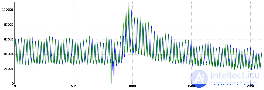
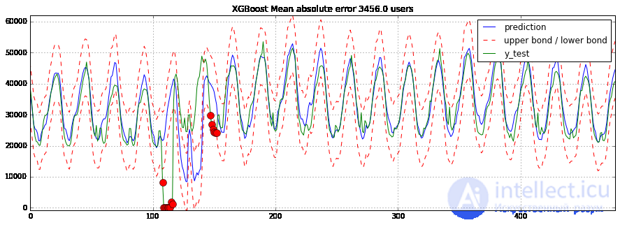
The same 3K users in mean absolute error, and anomalies caught fairly well on the test dataset. Of course, to reduce the error you could still tinker with the parameters, tune regularization if needed, select features, and figure out how many lags you need to go back into history, and so on.
We've gotten acquainted with various methods and approaches to analyzing and forecasting time series. Unfortunately, or fortunately, no silver bullet for solving this kind of problem has appeared yet. Methods developed in the 1960s (and some even earlier), are still just as popular as the LSTM or RNN methods not covered within this article. This is partly because the forecasting task, like any other task that arises when working with data — is largely creative and certainly exploratory. Despite the abundance of formal quality metrics and parameter estimation methods, for each time series you often have to search for and try something of your own. The balance between quality and effort also plays no small role. The SARIMA model, already mentioned here more than once, although it demonstrates outstanding results with proper tuning, may require more than an hour of tambourine-dancingmanipulations with the series, whereas a simple linear regression can be put together in 10 minutes, achieving more or less comparable results.
Current homework assignments are announced during each session of the course; you can follow along in the VK group and in the course repository.
In the demo version of the homework, you will be predicting the number of views of the "Machine Learning" wiki page. There is a web form for answers, where you will also find the solution.

Comments