
Lecture
Backpropagation through time (BPTT) is a gradient-based method for training certain types of recurrent neural networks . It can be used to train Elman networks . The algorithm was independently developed by numerous researchers.
The training data for a recurrent neural network is an ordered sequence of  input-output pairs,
  . An initial value
  must be specified for the hidden state. Usually a vector of all zeros is used for this purpose.
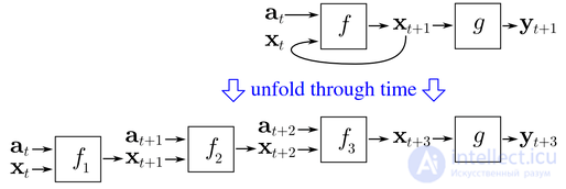
BPTT unrolls the recurrent neural network through time.
BPTT begins by unrolling the recurrent neural network through time. The unrolled network containsinputs and outputs, but all copies of the network share the same parameters. The backpropagation algorithm is then used to find the gradient of the cost with respect to all of the network's parameters.
Consider an example of a neural network containing a recurrent layer. and a feedforward layer
 . There are different ways of defining the training cost, but the total cost is always the average cost of each time step. The cost of each time step can be calculated separately. The figure above shows how the cost through time
 can be computed by unrolling the recurrent layer for three time steps and adding the feedforward layer . Every instance ofin the unrolled network has the same parameters. Thus, the weight update in each case (
 ) is summed.
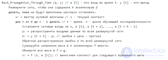
Pseudocode for a truncated version of BPTT, where the training data contains  input-output pairs, but the network is unrolled for time steps:
BPTT tends to be significantly faster for training recurrent neural networks than general-purpose optimization methods, such as evolutionary optimization.
BPTT has trouble with local optima. For recurrent neural networks, local optima are a much more serious problem than for feedforward neural networks. The periodic feedback in such networks tends to create chaotic responses on the error surface, which leads to local optima arising frequently, and in bad places on the error surface.
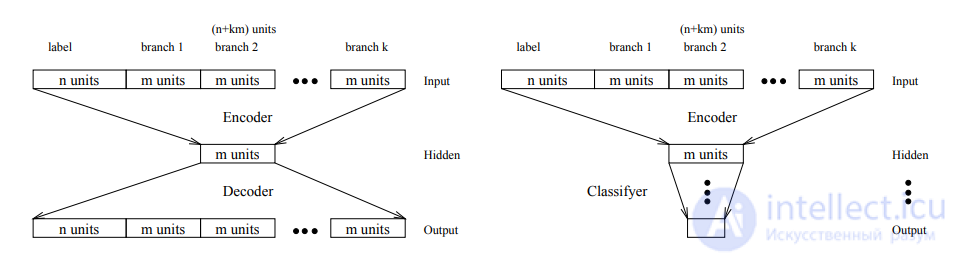
Figure 1: Standard LRAAM (A) and BPTS architecture (B).
Backpropagation Through Structure (BPTS) is a gradient-based method for training recursive neural networks (a superset of recurrent neural networks), which is described in detail in a 1996 paper written by Christoph Goller and Andreas Kuchler. Representing structures as DAGs. Let's first take a closer look at the way of encoding structures using Labeling Recursive Auto-Associative Memory (LRAAM) . All kinds of recursive symbolic data structures that we are aiming at can be mapped onto labeled directed acyclic graphs (DAGs), we do not consider cyclic structures here.. To compute the representation of a graph, one must first compute the representations of all subgraphs. During the LRAAM training stage, for each node one forward-propagation phase of activations and one backward-propagation phase (each through three levels of the network) of errors per epoch are needed. Choosing a DAG representation for structures, which allows representing different occurrences of a (sub)structure in the training set as only a single node, can lead to a significant (even exponential) reduction in the complexity of the standard LRAAM. This argument also holds for our architecture (see section 3). Instead of choosing a tree representation, we therefore prefer a DAG-like representation for our terms, as shown in Fig. 2.
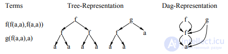
Figure 2: Tree and DAG representation of a set of terms.
For simplicity we will first restrict ourselves to tree-shaped structures. In the forward phase, the encoder (Fig. 1, B) is used to compute the representation for
a given tree in the same way as in the plain LRAAM. This is done by recursively feeding the previously computed representations of the direct subtrees into the encoder's input layer.
This encoding process starts at the leaves of the tree and generates the representation for the tree, which is then passed to the next layer, giving the classification result at the output of the Unit. The following metaphor helps us explain the backward phase. Imagine the encoder
virtually unrolled (with copied weights) according to the tree structure (see figure 3).
Now the error, passed from the classifier to the hidden layer, is propagated through the unrolled encoder network.
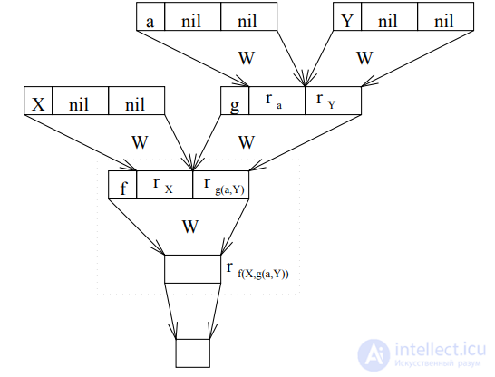
Figure 3: Encoding network unrolled by the structure f (X; g (a; Y)).
This unrolling by structure is analogous to unrolling a recurrent network through time (BPTT). It prompted us to introduce the term backpropagation through structure (BPTS). Let's first consider the case where a dedicated node in the training set is reserved for each occurrence of a (sub)term (tree representation). Arguing similarly to BPTT [Wer90], we see that the exact gradient is computed. Imagine that each copy of
part of the encoder has its own set of weights. Then, by the correctness of ordinary backpropagation, the exact gradient is computed. If the weight matrices of the different copies are identified, it is clear that we simply need to sum the components coming from the different copies to obtain
the exact gradient. The precise formulation is given below:
For each (sub)tree  is the encoder's input vector,
 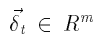 the delta (error) vector for representation t, and Q
(t: x; t') the projection of t: x onto the subtree t' of t
. Let further W be the encoder matrix, f' the derivative of the transfer function, and  the componentwise multiplication of two vectors.
Δ W is calculated as the sum over all (sub)trees (1).  for each subtree t' is calculated by propagating
  of one particular parent node t of t` back according to (2):

For each (sub)tree in the training set, exactly one forward and one
backward phase through the encoder is required per epoch. The training sample is static (there is no moving target).
However, if we use a DAG representation and represent a (sub)structure t as only a single node regardless of the number of its occurrences, there can be different  in (1) and (2) for each occurrence of t. We call this situation a delta conflict. Suppose that the (sub)structures ti and tj are identical. Of course, this means that the corresponding substructures within ti and tj are identical as well. This clearly gives us ti: x = tj: x, but we may have
To compute Δ W we will only need the sum  and
and 
. This is shown by the following transformation of (1), which holds because of the linearity of matrix multiplication:

 with the corresponding children t` of ti and tj can be computed more efficiently by propagating the sum
  and
and  back into (2). An analogous transformation (linearity of
  and matrix multiplication) for (2) shows this.
By summing all the differences arising in each case of the (sub)structure, we obtain the correct (steepest-gradient) resolution of the delta conflict and it allows a very efficient implementation of BPTS for DAGs. We simply need to arrange the nodes of the training set in topological order.
The forward phase starts at the leaf nodes and proceeds in reverse order, guaranteeing that representations for identical substructures need to be computed only once. The backward phase follows the topological order, starting from the root nodes.
Thus, the δ of all occurrences of a node are summed before that node is processed.. Again, for each node in the training set, exactly one forward and one backward phase through the encoder is required per epoch.
Like standard error backpropagation, BPTS can be used in batch or online mode. Batch BPTS updates the weights after the entire training set has been presented. By optimizing the methods discussed in Section 3 (delta summation and DAG representation), each node
only needs to be processed once per epoch. This is not the case for online mode, because the weights are updated immediately after a single structure is presented, and therefore substructures must be processed separately for each occurrence.

Comments