
Lecture
We have already gotten acquainted with several key machine learning algorithms. However, before moving on to more sophisticated algorithms and approaches, we would like to take a step aside and talk about preparing data for training a model. The well-known principle garbage in – garbage out applies 100% to any machine learning problem; any experienced analyst can recall examples from practice where a simple model trained on well-prepared data outperformed a sophisticated ensemble built on insufficiently clean data.

List of articles in the series
In today’s article, we would like to give an overview of three similar but different tasks:
Separately, note that this article will contain almost no formulas, but relatively a lot of code.
Some examples will use a dataset from the company Renthop, used in the Two Sigma Connect: Rental Listing Inquires competition on Kaggle. In this task, we need to predict the popularity of a rental listing, i.e. solve a three-class classification problem ['low', 'medium', 'high']. The solution is evaluated using the log loss metric (the lower — the better). Those who don’t yet have a Kaggle account will need to register; also, to download the data you need to accept the competition rules.
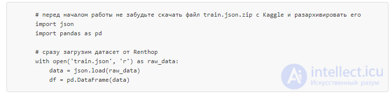
In real life, data rarely arrives in the form of ready-made matrices, so any task begins with feature extraction. Sometimes, of course, it is enough to read a csv file and convert it to numpy.array, but these are happy exceptions. Let’s look at some popular data types from which features need to be extracted.
Text – is the most obvious example of free-form data; there are enough methods for working with text that they would not fit into a single article. Nevertheless, let’s go over the most popular ones in an overview.
Before working with text, it needs to be tokenized. Tokenization means splitting the text into tokens – in the simplest case these are just words. But if we do this with an overly simple regex (a "brute-force" one), we can lose part of the meaning: "Nizhny Novgorod" is not two tokens but one. On the other hand, the slogan "steal-and-kill!" could be mistakenly split into two tokens. There are ready-made tokenizers that account for the specifics of the language, but even they can make mistakes, especially if you are working with specific texts (professional vocabulary, jargon, typos).
After tokenization, in most cases you need to think about bringing words to their normal form. This refers to stemming and/or lemmatization – similar processes used to process word forms. You can read about the difference between them here.
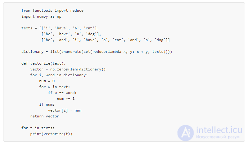
So, we have turned the document into a sequence of words, and now we can start turning them into vectors. The simplest approach is called Bag of Words: we create a vector as long as the vocabulary, count the number of occurrences of each word in the text, and put this number into the corresponding position in the vector. In code this looks even simpler than in words:
Bag of Words without extra libraries
The idea is also nicely illustrated by a picture:
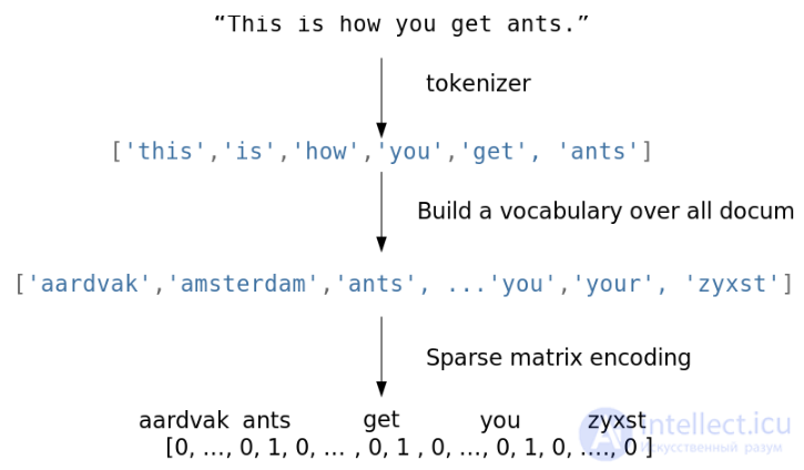
This is an extremely naive implementation. In real life you need to take care of stop words, the maximum vocabulary size, and an efficient data structure (text data is usually turned into sparse vectors)…
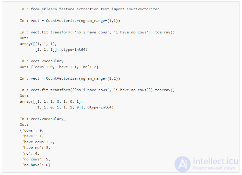
Using algorithms like Bag of Words, we lose the order of words in the text, which means that the texts "i have no cows" and "no, i have cows" will be identical after vectorization, even though they are semantically opposite. To avoid this problem, you can take a step back and change the approach to tokenization: for example, use N-grams (combinations of N consecutive terms).
Let’s check this in practice
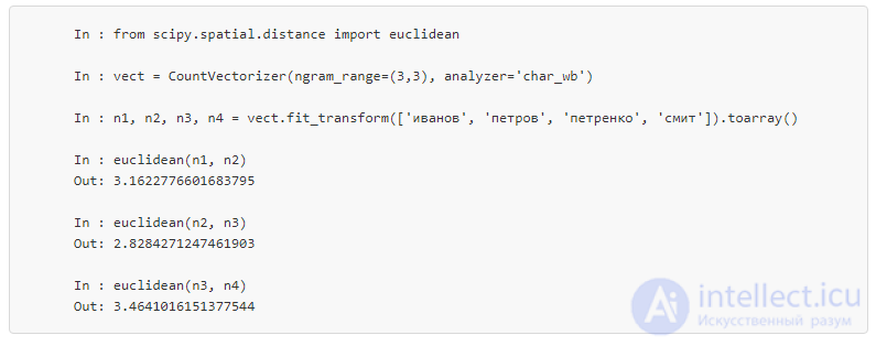
I’ll also note that it is not necessary to operate on words specifically: in some cases you can generate N-grams from letters (for example, such an algorithm will account for the similarity of related words or typos).
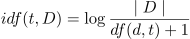
An extension of the Bag of Words idea: words that are rare in the corpus (across all the documents considered in this dataset) but present in this particular document may turn out to be more important. In that case it makes sense to increase the weight of more narrowly-themed words in order to separate them from general-topic words. This approach is called TF-IDF, and it can no longer be written in ten lines, so those interested can look into the details in external sources such as wiki. The default variant looks like this:

Analogs of Bag of words can also be found outside of text tasks: for example, bag of sites in the competition we run – Catch Me If You Can. You can also look for other examples – bag of apps, bag of events.
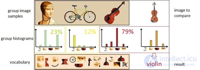
Using such algorithms, you can get a quite workable solution to a simple problem, a kind of baseline. However, for those who are not fans of the classics, there are also newer approaches. The most hyped method of the new wave – Word2Vec, but there are also alternatives (Glove, Fasttext…).
Word2Vec is a special case of Word Embedding algorithms. Using Word2Vec and similar models, we can not only vectorize words into a high-dimensional space (usually several hundred), but also compare their semantic closeness. A classic example of operations on vectorized representations: king – man + woman = queen.
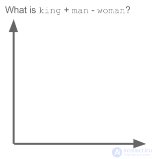
It’s worth understanding that this model, of course, does not have an understanding of words, but simply tries to place vectors in such a way that words used in a common context are placed close to each other. If this is not taken into account, you can come up with many curiosities: for example, finding the opposite of Hitler by multiplying the corresponding vector by -1.
Such models need to be trained on very large datasets so that the coordinates of the vectors truly reflect the semantics of the words. To solve your own tasks, you can download a pretrained model, for example, here.
Similar methods, by the way, are also used in other fields (for example, in bioinformatics). One of the most unexpected applications – food2vec.
Working with images is both simpler and more complicated at the same time. Simpler, because often you don’t need to think at all and can just use one of the popular pretrained networks; more complicated, because if you actually need to dig into the details, this rabbit hole turns out to be damn deep. However, let’s take things in order.
Back when GPUs were weaker and the "neural network renaissance" had not yet happened, generating features from images was a separate, complex field. Working with images required working at a low level, determining, for example, edges, region boundaries, and so on. Specialists experienced in computer vision could draw many parallels between older approaches and neural-network hipsterism: in particular, convolutional layers in modern networks are very similar to Haar cascades. Not being experienced in this area, I won’t even try to convey the knowledge from public sources, I’ll just leave a couple of links to the skimage and SimpleCV libraries and move straight on to our days.
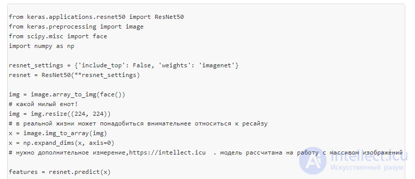
Often, for tasks related to images, some kind of convolutional network is used. Instead of coming up with an architecture and training a network from scratch, you can take a pretrained state of the art network whose weights can be downloaded from open sources. To adapt it to your own task, data scientists practice so-called fine tuning: the network’s last fully-connected layers are "torn off", and new ones tailored to the specific task are added in their place, then the network is retrained on the new data. But if you just want to vectorize an image for some purpose of your own (for example, to use some non-network classifier) – simply tear off the last layers and use the output of the previous layers:
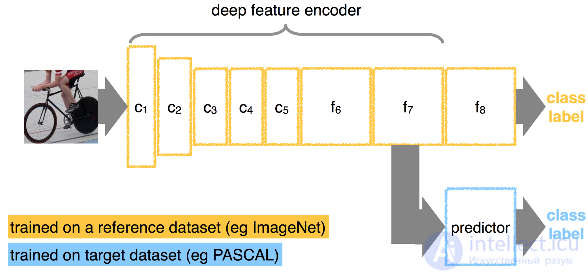
A classifier trained on one dataset and adapted for another by "tearing off" the last layer and adding a new one in its place
Nevertheless, it is not worth fixating solely on neural-network methods. Some hand-crafted features can still be useful today: for example, when predicting the popularity of apartment rental listings, you could assume that bright apartments attract more attention, and create a "mean pixel value" feature. You can find inspiration for examples in the documentation of the corresponding libraries.
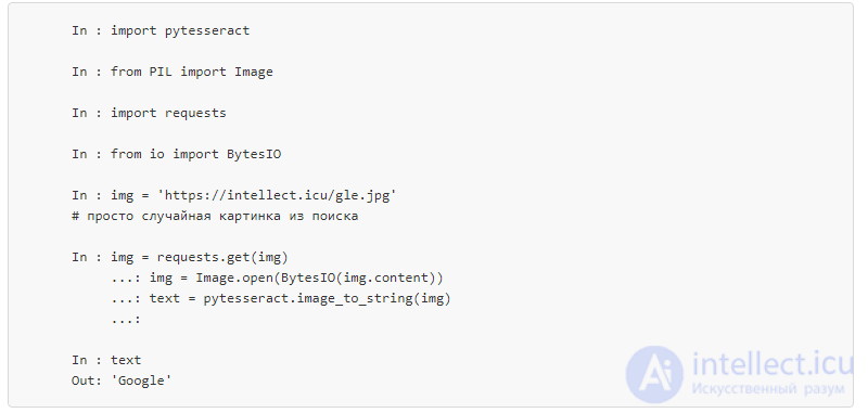
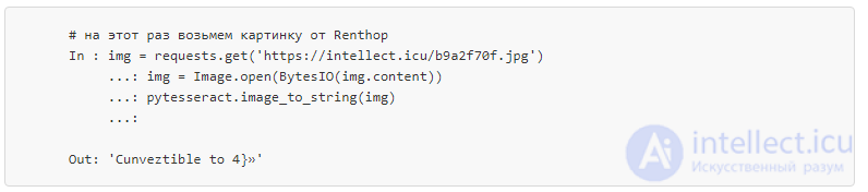
If text is expected in the image, it can also be read without building a complex neural network yourself: for example, using pytesseract.
You need to understand that pytesseract – is far from a panacea:
Another case where neural networks won’t help – extracting features from metainformation. And EXIF can actually store a lot of useful data: camera manufacturer and model, resolution, flash usage, shooting geocoordinates, the software used for processing, and much more.
Geographic data doesn’t come up in tasks all that often, but it is also useful to master the basic techniques for working with it, especially since there are plenty of ready-made solutions in this area as well.
Geodata is most often represented as addresses or "latitude + longitude" pairs, i.e. points. Depending on the task, you may need two operations that are the inverse of each other: geocoding (recovering a point from an address) and reverse geocoding (the opposite). Both are achievable using external APIs such as Google Maps or OpenStreetMap. Different geocoders have their own quirks, and quality varies from region to region. Fortunately, there are universal libraries such as geopy, which act as wrappers over a number of external services.
If there is a lot of data, it is easy to run into the limits of external APIs. And retrieving information over HTTP – is not always the fastest solution either. So it is worth keeping in mind the possibility of using a local version of OpenStreetMap.
If there isn’t much data, there is enough time, and you don’t feel like extracting fancy features, you don’t need to bother with OpenStreetMap and can use reverse_geocoder instead:
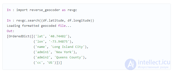
When working with geocoding, you must not forget that addresses can contain typos, so it is worth spending time on cleaning them up. Coordinates usually have fewer typos, but they are not free of problems either: by its nature GPS data can "be noisy", and in some places (tunnels, skyscraper blocks...) – quite noticeably so. If the data source – is a mobile device, keep in mind that in some cases location is determined not by GPS but by nearby WiFi networks, which leads to holes in space and teleportation: among a set of points describing a trip across Manhattan, one might suddenly turn out to be from Chicago.
Hypotheses about teleportation
WiFi location tracking is based on a combination of SSID and MAC address, which can coincide for completely different points (for example, a federal provider standardized router firmware down to the MAC address and deploys them in different cities). There are also more mundane reasons, such as a company moving with its own routers to another office.
A point is usually not located in an open field but among infrastructure – here you can let your imagination run wild and start coming up with features, drawing on life experience and domain knowledge. Proximity of the point to a subway station, building density, distance to the nearest store, number of ATMs within a radius – within a single task you can come up with dozens of features and obtain them from various external sources. For tasks outside urban infrastructure, features from more specific sources may come in handy: for example, elevation above sea level.
If two or more points are related, it may be worth extracting features from the route between them. Distances are useful here (it’s worth looking at both the great circle distance and the "honest" distance calculated over the road graph), as well as the number of turns together with the ratio of left to right turns, and the number of traffic lights, interchanges, and bridges. For example, in one of my tasks, a feature I called "road complexity" performed quite well – distance calculated over the graph and divided by the GCD.
You would think that working with date and time should be standardized given how common the corresponding features are, but there are still pitfalls.
Let’s start with days of the week – they can easily be turned into 7 dummy variables using one-hot encoding. In addition, it is useful to single out a separate feature for weekends.

Some tasks may require additional calendar features: for example, cash withdrawals may be tied to payday, while buying a transit pass – to the start of the month. Ideally, when working with time-based data, you should have on hand a calendar of public holidays, anomalous weather conditions, and other important events.
Professional unfunny humor

But with the hour (minute, day of the month...) things are not so rosy. If you use the hour as a continuous variable, we somewhat contradict the nature of the data: 0 < 23, even though 02.01 0:00:00 > 01.01 23:00:00. For some tasks this can turn out to be critical. If, on the other hand, you encode them as categorical variables, you can end up with a pile of features and lose information about proximity: the difference between 22 and 23 will be the same as between 22 and 7.
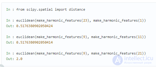
There are also more esoteric approaches to such data. For example, projecting onto a circle followed by using the two coordinates.
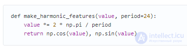
Such a transformation preserves the distance between points, which is important for some distance-based algorithms (kNN, SVM, k-means...)
However, the difference between such encoding methods can usually only be noticed at the third decimal place of the metric, not earlier.
I haven’t had the chance to work extensively with time series, so I will leave a link to a library for automatic feature generation from time series and move on.
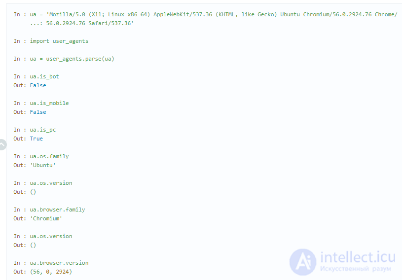
If you work with the web, you usually have information about the user’s User Agent. This is a treasure trove of information.
First of all, you need to extract the operating system from it. Second, create an is_mobile feature. Third, look at the browser.
Example of feature extraction from a user agent
As with other domain areas, you can come up with your own features based on guesses about the nature of the data. At the time this article was written, Chromium 56 was new, and after some time such a browser version will only remain with those who haven’t restarted this very browser in a very long time. So why not introduce a feature such as "lag behind the latest browser version"?
In addition to the OS and browser, you can look at the referer (not always available), http_accept_language, and other metadata.
The next most useful piece of information – is the IP address, from which you can extract at least the country, and preferably also the city, provider, and connection type (mobile / stationary). You need to understand that there are various proxies and outdated databases, so the feature may contain noise. Network administration gurus can try extracting much fancier features: for example, making assumptions about VPN usage. By the way, data from the IP address combines well with http_accept_language: if a user is sitting behind a Chilean proxy while the browser locale – is ru_RU, something is off here and deserves a one in the corresponding column of the table (is_traveler_or_proxy_user).
In general, there is so much domain specificity in one area or another that it can’t fit in a single head. That is why I encourage the respected readers to share their experience and talk in the comments about extracting and generating features in their own work.
A monotonic transformation of features is critical for some algorithms and has no effect on others. By the way, this is one of the reasons for the popularity of decision trees and all their derivative algorithms (random forest, gradient boosting) – not everyone is able to or wants to bother with transformations, and these algorithms are robust to unusual distributions.
There are also purely engineering reasons: np.log as a way to deal with numbers too large to fit into np.float64. But this is more the exception than the rule; more often it is caused by the desire to adapt the dataset to the algorithm’s requirements. Parametric methods usually require at least a symmetric and unimodal data distribution, which the real world doesn’t always provide. There can be even stricter requirements (it’s worth recalling the lesson on linear models).
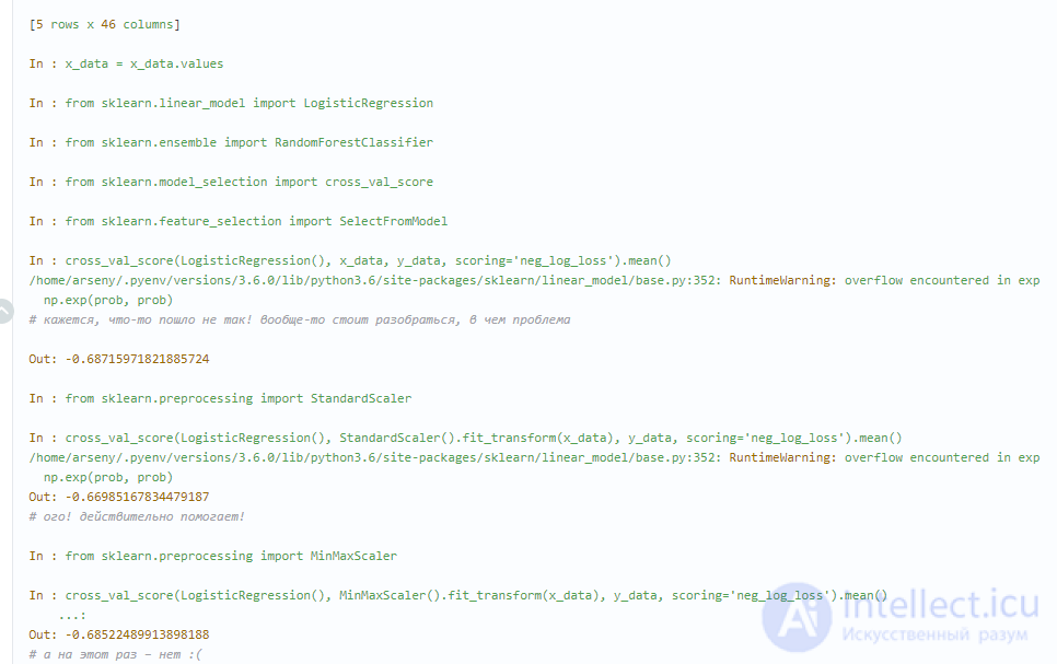
However, it’s not only parametric methods that impose requirements on the data: the same nearest neighbors method will predict complete nonsense if the features are not normalized: one distribution sits around zero and doesn’t go beyond (-1, 1), while another feature – is in the hundreds and thousands.
A simple example: suppose the task is to predict the price of an apartment from two features – distance from the center and number of rooms. The number of rooms rarely exceeds 5, while the distance from the center in large cities can easily be measured in tens of thousands of meters.
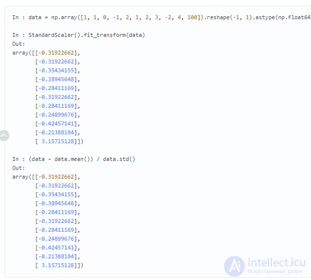
The simplest transformation – is Standart Scaling (also known as Z-score normalization).

Although StandartScaling doesn’t make the distribution normal in the strict sense of the word...
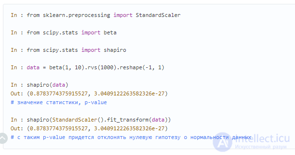
… it does provide some protection against outliers
Another fairly popular option – is MinMax Scaling, which maps all points onto a given interval (usually (0, 1)).
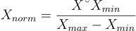
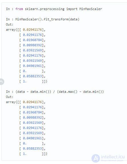
StandartScaling and MinMax Scaling have similar areas of applicability and are often more or less interchangeable. However, if the algorithm involves computing distances between points or vectors, the default choice – is StandartScaling. On the other hand, MinMax Scaling is useful for visualization, to map features onto the interval (0, 255).
If we assume that some data is not normally distributed, but is instead described by a lognormal distribution, it can easily be brought to a genuinely normal distribution:
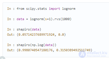
A lognormal distribution is suitable for describing salaries, the value of securities, city populations, the number of comments on articles on the internet, and so on. However, for this technique to apply, the distribution does not necessarily have to be exactly lognormal – any distribution with a heavy right tail can be tried with this kind of transformation. In addition, you can try applying other similar transformations, guided by your own hypotheses about how to bring the existing distribution closer to normal. Examples of such transformations are the Box-Cox transformation (taking the logarithm – is a special case of the Box-Cox transformation) or the Yeo-Johnson transformation, which extends the applicability to negative numbers; in addition, you can simply try adding a constant to the feature – np.log(x + const).
In the examples above we worked with synthetic data and strictly checked for normality using the Shapiro-Wilk test. Let’s try to look at real data, and to check for normality we will use a less formal method – the Q-Q plot. For a normal distribution it will look like a straight diagonal line, and visual deviations are intuitively easy to understand.
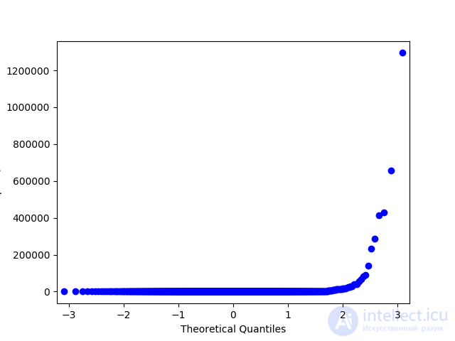
Q-Q plot for a lognormal distribution
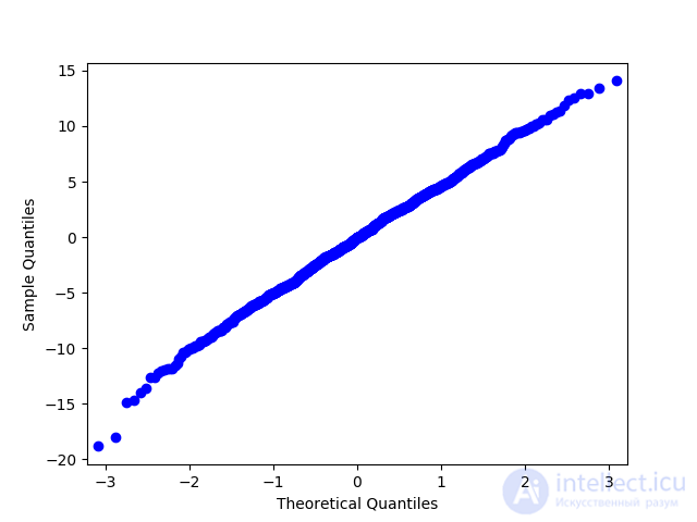
Q-Q plot for the same distribution after taking the logarithm
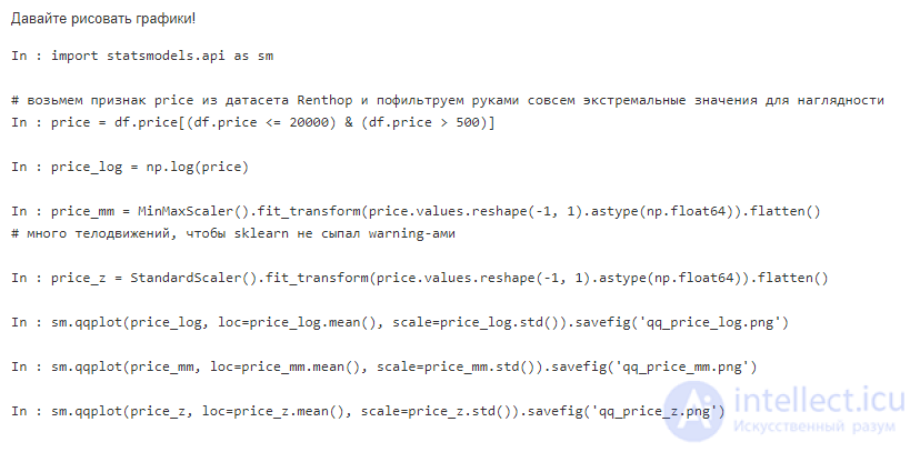
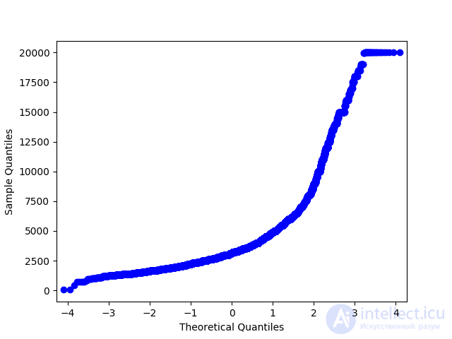
Q-Q plot of the original feature
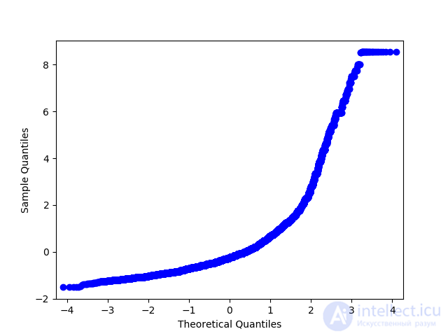
Q-Q plot of the feature after StandartScaler. The shape doesn’t change
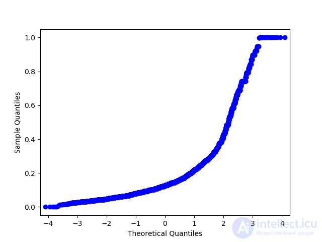
Q-Q plot of the feature after MinMaxScaler. The shape doesn’t change
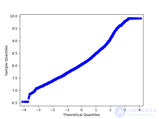
Q-Q plot of the feature after taking the logarithm. Things are looking better now!
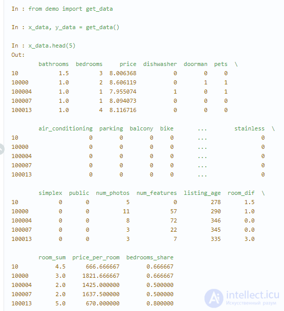
Let’s see whether transformations can somehow help a real model. I made a small script that reads the data from the Renthop competition, selects some features (the rest are dictatorially dropped for simplicity), and returns us more or less ready-made data for the demonstration.
If the previous transformations were dictated more by mathematics, this point is again justified by the nature of the data; it can be attributed both to transformations and to the creation of new features.
Let’s turn again to the Two Sigma Connect: Rental Listing Inquires task. Among the features in this task are the number of rooms and the rental price. Everyday logic suggests that the price per room is more informative than the total price – so it might be worth trying to single out such a feature.

It is not necessary to be guided by everyday logic. If there aren’t too many features, you can quite well generate all possible interactions and then filter out the unnecessary ones using one of the techniques described in the next section. Moreover, not all interactions between features need to have any physical meaning at all: for example, (often used for linear models)[https://habrahabr.ru/company/ods/blog/322076/] polynomial features (see sklearn.preprocessing.PolynomialFeatures) are practically impossible to interpret.
Not many algorithms can work with missing values "out of the box", and the real world often supplies data with gaps. Fortunately, this is one of those tasks that requires no creativity at all to solve. Both of the key python libraries for data analysis provide solutions as simple as can be: pandas.DataFrame.fillna and sklearn.preprocessing.Imputer.
Ready-made library solutions don’t hide any magic behind their facade. Approaches to handling missing values suggest themselves at the level of common sense:
The convenience of ready-made library solutions sometimes tempts you to just stick in something like df = df.fillna(0) and not worry about the missing values. But this is not the wisest decision: most of the time is usually spent not on building the model, but on preparing the data; thoughtless implicit filling of missing values can hide a bug in the processing and ruin the model.
Why would you even need to select features? To some this idea might seem counterintuitive, but in fact there are at least two important reasons to get rid of unimportant features. The first is clear to any engineer: the more data, the higher the computational complexity. As long as we’re playing around with toy datasets, the size of the data – is not a problem, but for a real heavily loaded production system, a few hundred extra features can be noticeable. The other reason – is that some algorithms mistake noise (uninformative features) for signal, overfitting as a result.
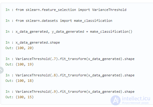
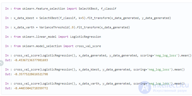
The most obvious candidate for removal – is a feature whose value never changes, i.e. contains no information at all. If we step a little away from this degenerate case, it is reasonable to assume that low-variance features are generally worse than high-variance ones. This leads to the idea of discarding features whose variance is below a certain threshold.
There are also other methods, also based on classical statistics.
You can see that the selected features improved the classifier’s quality. It’s clear that this example is purelysynthetic, but nevertheless the technique deserves to be tested on real tasks as well.
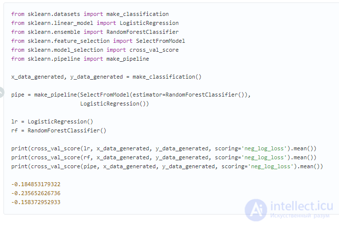
Another approach: use some baseline model to evaluate the features, where the model must explicitly show the importance of the features used. Usually two types of models are used: some kind of "tree-based" ensemble (for example, Random Forest) or a linear model with Lasso regularization, which tends to zero out the weights of weak features. The logic is intuitively clear: if features are clearly useless in a simple model, there’s no need to drag them along into a more complex one either.
Synthetic example
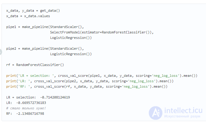
We must not forget that this is also not a silver bullet — it can even turn out worse.
Let’s go back to the Renthop dataset.
Finally, the most reliable, but also the most computationally expensive method is based on a plain brute-force search: we train a model on a subset of "features", remember the result, repeat for different subsets, and compare the quality of the models. This approach is called Exhaustive Feature Selection.
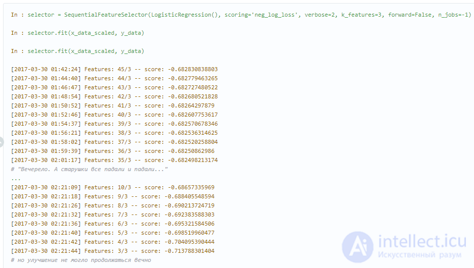
Trying out all combinations – is usually too slow, so you can try to reduce the search space. We fix a small number N, go through all combinations of N features, choose the best combination, then go through combinations of N+1 features such that the previous best combination of features is fixed and only the new feature varies. This way you can keep going until you hit the maximum allowed number of features or until the model’s quality stops improving significantly. This algorithm is called Sequential Feature Selection.
This same algorithm can be reversed: start with the full feature space and discard features one at a time, as long as this doesn’t hurt the model’s quality or until the desired number of features is reached.
Time for a leisurely brute-force search!

Comments