
Lecture
Let's talk about machine learning problems and look at 2 simple approaches – decision trees and the nearest neighbors method.
We will also discuss how to use cross-validation to select a model for specific data.
Plan:
You probably want to jump right into the fray, but first let's talk about exactly what problem we will be solving and what its place is in the field of machine learning.
The classic, general (and not particularly rigorous) definition of machine learning goes like this (T. Mitchell "Machine learning", 1997):
a computer program is said to learn when solving some task from class T, if its performance, according to metric P, improves with the accumulation of experience E.
Further on, in different scenarios, T, P, and E refer to completely different things. Among the most popular T tasks in machine learning are:
By experience E we mean data (there's no doing without it), and depending on this, machine learning algorithms can be divided into those that learn with a teacher and without a teacher (supervised & unsupervised learning). In unsupervised learning problems there is a sample consisting of objects described by a set of features. In supervised learning problems, in addition to this, for each object of a certain sample, called the training sample, a target feature is known – essentially this is what we would like to predict for other objects that are not in the training sample.
Example
Classification and regression problems are supervised learning problems. As an example, we will use the credit scoring problem: based on data accumulated by a lending institution about its clients, we want to predict loan default. Here, for the algorithm, the experience E is the available training sample: a set of objects (people), each of which is characterized by a set of features (such as age, salary, loan type, past defaults, etc.), as well as a target feature. If this target feature is simply the fact of loan default (1 or 0, i.e. the bank knows about its clients which ones repaid the loan and which did not), then this is a (binary) classification problem. If it is known by how much in time the client was late in repaying the loan, and we want to predict the same thing for new clients, then this will be a regression problem.
Finally, the third abstraction in the definition of machine learning is the algorithm's performance metric P. Such metrics differ for different tasks and algorithms, and we will talk about them as we study the algorithms. For now, let's just say that the simplest quality metric for an algorithm solving a classification problem is the fraction of correct answers (accuracy, do not call it correctness – that term is reserved for a different metric, precision) – that is, simply the fraction of the algorithm's correct predictions on the test set.
Next we will talk about two supervised learning problems: classification and regression.
Let's begin our overview of classification and regression methods with one of the most popular ones – the decision tree. Decision trees are used in everyday life in a wide variety of areas of human activity, sometimes far removed from machine learning. A decision tree can be thought of as a visual set of instructions on what to do in a given situation. Let's give an example from the field of advising research staff at an institute. The Higher School of Economics publishes info-diagrams that make life easier for its employees. Here is a fragment of the instructions for publishing a scientific paper on the institute's portal.
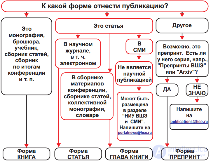
In terms of machine learning, we can say that this is an elementary classifier that determines the form of a publication on the portal (book, article, book chapter, preprint, publication in "HSE and the Media") based on several features: publication type (monograph, brochure, article, etc.), the type of publication venue where the article was published (scientific journal, proceedings, etc.), and others.
Quite often a decision tree serves as a generalization of expert experience, a means of passing knowledge on to future employees, or a model of a company's business process. For example, before scalable machine learning algorithms were introduced in banking, the credit scoring problem was solved by experts. The decision on whether to grant a loan to a borrower was made based on some intuitively (or empirically) derived rules, which can be represented as a decision tree.
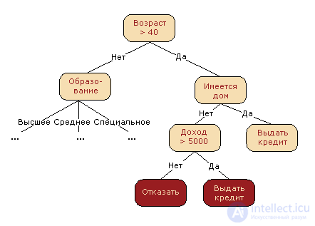
In this case, we can say that a binary classification problem is being solved (the target class has two values: "Grant the loan" and "Decline") based on the features "Age", "Home ownership", "Income", and "Education".
A decision tree as a machine learning algorithm is essentially the same thing: combining logical rules of the form "Value of feature a is less than x AND Value of feature b is less than y… => Class 1" into a "Tree" data structure. A huge advantage of decision trees is that they are easily interpretable and understandable to a human. For example, using the diagram in the figure above, one can explain to a borrower why they were denied a loan. Say, because they don't own a home and their income is less than 5000. As we will see further on, many other, though more accurate, models do not have this property and can rather be regarded as a "black box" into which data was loaded and an answer was obtained. Because of this "understandability" of decision trees and their similarity to the human decision-making model (you can easily explain your model to your boss), decision trees have become extremely popular, and one of the representatives of this group of classification methods, C4.5, is ranked first in the list of the top 10 algorithms in data mining ("Top 10 algorithms in data mining", Knowledge and Information Systems, 2008. PDF).
In the credit scoring example, we saw that the decision to grant a loan was made based on age, property ownership, income, and other factors. But which feature should be chosen first? To answer this, let's consider a simpler example, where all features are binary.
Here we can recall the game "20 questions", which is often mentioned in introductions to decision trees. Surely everyone has played it. One person thinks of a celebrity, and the other tries to guess who it is by asking only questions that can be answered "Yes" or "No" (let's leave aside the options "I don't know" and "I can't say"). Which question will the guesser ask first? Of course, the one that will most strongly reduce the number of remaining options. For example, the question "Is it Angelina Jolie?", if answered negatively, will leave more than 7 billion options for further consideration (of course, somewhat fewer, since not every person is a celebrity, but still quite a lot), whereas the question "Is it a woman?" will already cut off about half of the celebrities. That is, the feature "gender" splits the sample of people much better than the feature "is it Angelina Jolie", "nationality-Spanish", or "likes football". This intuitively corresponds to the concept of information gain, based on entropy.
Entropy
Shannon entropy is defined for a system with N possible states as follows:
S=−∑i=1Npilog2pi,
where pi – is the probability of finding the system in the i-th state. This is a very important concept, used in physics, information theory, and other fields. Skipping the derivation (combinatorial and information-theoretic) of this concept, let's note that, intuitively, entropy corresponds to the degree of chaos in a system. The higher the entropy, the less ordered the system, and vice versa. This will help us formalize the "effective splitting of the sample" that we talked about in the context of the "20 questions" game.
Example
To illustrate how entropy helps determine good features for building a tree, let's give the same toy example as in the article "Entropy and decision trees". We will predict the color of a ball from its coordinate. Of course, this has nothing to do with real life, but it allows us to show how entropy is used to build a decision tree.

Here there are 9 blue balls and 11 yellow ones. If we draw a ball at random, it will be blue with probability p1=920 and yellow with probability p2=1120 – . This means the entropy of state S0=−920log2920−1120log21120≈1. By itself this value doesn't tell us anything yet. Now let's see how the entropy changes if we split the balls into two groups – with coordinate less than or equal to 12, and greater than 12.
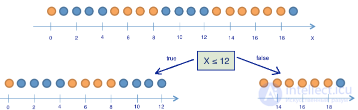
In the left group there turned out to be 13 balls, of which 8 are blue and 5 are yellow. The entropy of this group is S1=−513log2513−813log2813≈0.96. In the right group there turned out to be 7 balls, of which 1 is blue and 6 are yellow. The entropy of the right group is S2=−17log217−67log267≈0.6. As we can see, entropy decreased in both groups compared to the initial state, though not by much in the left one. Since entropy is essentially the degree of chaos (or uncertainty) in a system, a decrease in entropy is called information gain. Formally, the information gain (IG) when splitting the sample by feature Q (in our example this is the feature "x≤12") is defined as
IG(Q)=SO−∑i=1qNiNSi,
where q – is the number of groups after splitting, Ni – is the number of sample elements for which feature Q has the i-th value. In our case, after splitting we got two groups (q=2) – one of 13 elements (N1=13), the second – of 7 (N2=7). The information gain turned out to be
IG(x≤12)=S0−1320S1−720S2≈0.16.
It turns out that by splitting the balls into two groups by the feature "coordinate less than or equal to 12", we have already obtained a more ordered system than at the start. Let's continue splitting the balls into groups until the balls in each group are of the same color.
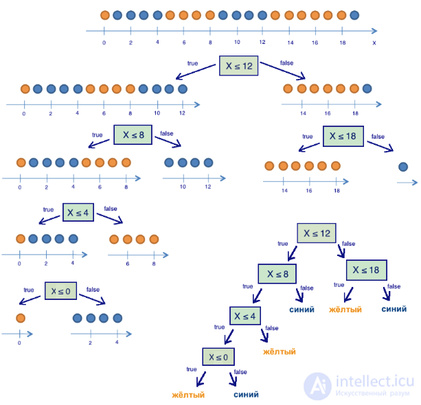
For the right group, just one additional split was needed by the feature "coordinate less than or equal to 18", for the left group – three more. Obviously, the entropy of a group of balls of the same color is 0 (log21=0), which matches the intuition that a group of balls of a single color is ordered.
As a result, we have built a decision tree that predicts the color of a ball from its coordinate. Note that such a decision tree may work poorly for new objects (determining the color of new balls), since it has perfectly fitted itself to the training sample (the original 20 balls). For classifying new balls, a tree with fewer "questions", or splits, would be better suited, even if it does not split the training sample perfectly by color. We will look at this problem, overfitting, further on.
We can verify that the tree built in the previous example is, in some sense, optimal – only 5 "questions" (conditions on feature x) were needed to "fit" the decision tree to the training sample, that is, so that the tree correctly classifies any training object. Under different sample-splitting conditions, the tree would turn out deeper.
The popular decision tree building algorithms, such as ID3 and C4.5, are based on the principle of greedy maximization of information gain – at each step, the feature is chosen for which splitting yields the greatest information gain. The procedure is then repeated recursively until the entropy turns out to be zero or some small value (if the tree is not fit perfectly to the training sample, in order to avoid overfitting).
Different algorithms use different heuristics for "early stopping" or "pruning" to avoid building an overfitted tree.
def build(L):
    create node t
    if the stopping criterion is True:
        assign a predictive model to t
    else:
        Find the best binary split L = L_left + L_right
        t.left = build(L_left)
        t.right = build(L_right)
    return t
We have seen how the concept of entropy allows us to formalize the notion of split quality in a tree. But this is just one heuristic; there are others:
In practice, the misclassification error is almost never used, while Gini impurity and information gain work almost identically.
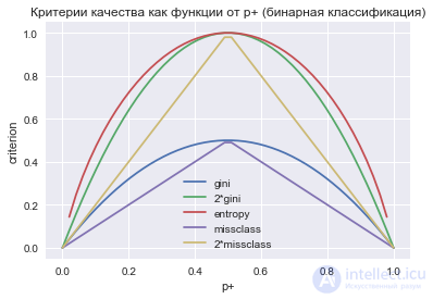
For a binary classification problem (p+ – the probability of an object having the label +), entropy and Gini impurity take the following form:
S=−p+log2p+−p−log2p−=−p+log2p+−(1−p+)log2(1−p+);
G=1−p+2−p−2=1−p+2−(1−p+)2=2p+(1−p+).
When we plot these two functions of the argument p+, we will see that the entropy graph is very close to the graph of twice the Gini impurity, and therefore in practice these two criteria "work" almost identically.
Importing libraries
from __future__ import division, print_function
# turn off all the Anaconda warnings
import warnings
warnings.filterwarnings('ignore')
import numpy as np
import pandas as pd
%matplotlib inline
import seaborn as sns
from matplotlib import pyplot as plt
Plotting the figure
plt.rcParams['figure.figsize'] = (6,4)
xx = np.linspace(0,1,50)
plt.plot(xx, [2 * x * (1-x) for x in xx], label='gini')
plt.plot(xx, [4 * x * (1-x) for x in xx], label='2*gini')
plt.plot(xx, [-x * np.log2(x) - (1-x) * np.log2(1 - x)  for x in xx], label='entropy')
plt.plot(xx, [1 - max(x, 1-x) for x in xx], label='missclass')
plt.plot(xx, [2 - 2 * max(x, 1-x) for x in xx], label='2*missclass')
plt.xlabel('p+')
plt.ylabel('criterion')
plt.title('Quality criteria as functions of p+ (binary classification)')
plt.legend();
Example
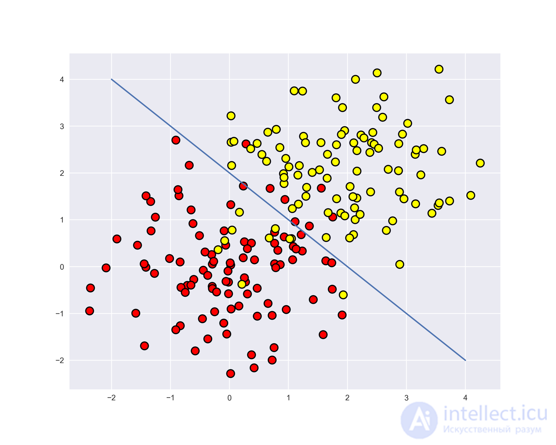
Let's look at an example of applying a decision tree from the Scikit-learn library to synthetic data. Two classes will be generated from two normal distributions with different means.
Code for generating the data
# first class
np.seed = 7
train_data = np.random.normal(size=(100, 2))
train_labels = np.zeros(100)

# add the second class
train_data = np.r_[train_data, np.random.normal(size=(100, 2), loc=2)]
train_labels = np.r_[train_labels, np.ones(100)]
Let's plot the data. Informally, the classification problem in this case is to construct some "good" boundary separating the 2 classes (red dots from yellow ones). To simplify, machine learning in this case comes down to how to choose a good separating boundary. Perhaps a straight line will be too simple a boundary, while some complex curve enveloping every red dot will be too complex, and we will make a lot of mistakes on new examples from the same distribution that the training sample came from. Intuition suggests that some smooth boundary separating the 2 classes, or at least simply a straight line (in the n-dimensional case – a hyperplane), will work well on new data.
Plotting the figure
plt.rcParams['figure.figsize'] = (10,8)
plt.scatter(train_data[:, 0], train_data[:, 1], c=train_labels, s=100,
cmap='autumn', edgecolors='black', linewidth=1.5);
plt.plot(range(-2,5), range(4,-3,-1));
Let's try to separate these two classes by training a decision tree. In the tree, we'll use the parameter max_depth, which limits the depth of the tree. Let's visualize the resulting class separation boundary.
Code for training the tree and plotting its separating boundary
from sklearn.tree import DecisionTreeClassifier

# Let's write a helper function that will return a grid for further visualization.
def get_grid(data):
    x_min, x_max = data[:, 0].min() - 1, data[:, 0].max() + 1
    y_min, y_max = data[:, 1].min() - 1, data[:, 1].max() + 1
    return np.meshgrid(np.arange(x_min, x_max, 0.01), np.arange(y_min, y_max, 0.01))

# the min_samples_leaf parameter specifies the minimum number of
# elements in a node for it to be split further
clf_tree = DecisionTreeClassifier(criterion='entropy', max_depth=3, random_state=17)

# train the tree
clf_tree.fit(train_data, train_labels)

# a bit of code to display the separating surface
xx, yy = get_grid(train_data)
predicted = clf_tree.predict(np.c_[xx.ravel(), yy.ravel()]).reshape(xx.shape)
plt.pcolormesh(xx, yy, predicted, cmap='autumn')
plt.scatter(train_data[:, 0], train_data[:, 1], c=train_labels, s=100,
cmap='autumn', edgecolors='black', linewidth=1.5);
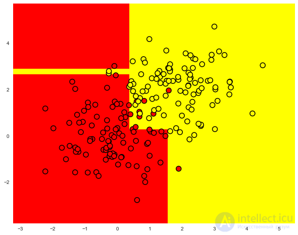
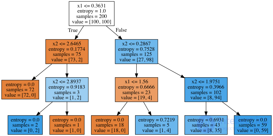
What does the resulting tree itself look like? We see that the tree "slices" the space into 7 rectangles (the tree has 7 leaves). Within each such rectangle, the tree's prediction will be constant, based on the prevalence of objects of one class or the other.
Code for displaying the tree
How is such a tree "read"?
At the start there were 200 objects, 100 — of one class and 100 – of the other. The entropy of the initial state was maximal – 1. Then the objects were split into 2 groups depending on comparing feature x1 with the value 0.3631 (find this section of the boundary in the figure above, before the tree). In this case, entropy decreased in both the left and the right group of objects. And so on, the tree is built up to a depth of 3. In this visualization, the more objects of one class there are, the closer the node's color is to dark orange, and conversely, the more objects of the second class there are, the closer the color is to dark blue. At the start there is an equal number of objects of each class, so the root node of the tree is white.
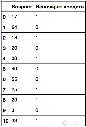
Suppose the sample has a quantitative feature "Age" with many unique values. The decision tree will look for the best split of the sample (by a criterion such as information gain), checking binary features like "Age < 17", "Age < 22.87", etc. But what if there are too many such age "cuts"? And what if there is also a quantitative feature "Salary", and salary can also be "cut" in many ways? It turns out there are too many binary features to choose the best one at each step of building the tree. To solve this problem, heuristics are used to limit the number of thresholds against which we compare a quantitative feature.
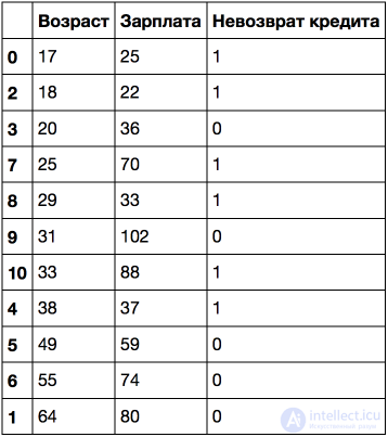
Let's consider this with a toy example. Suppose we have the following sample:
Let's sort it by increasing age.
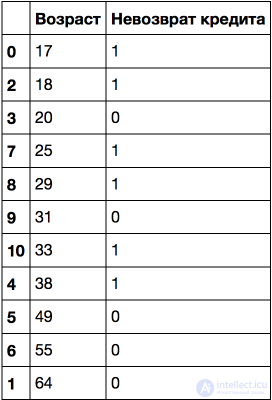
Let's train a decision tree on this data (without limiting the depth) and take a look at it.
Code for training and plotting the tree
age_tree = DecisionTreeClassifier(random_state=17)
age_tree.fit(data['Возраст'].values.reshape(-1, 1), data['Невозврат кредита'].values)

export_graphviz(age_tree, feature_names=['Возраст'],
out_file='../../img/age_tree.dot', filled=True)
!dot -Tpng '../../img/age_tree.dot' -o '../../img/age_tree.png'
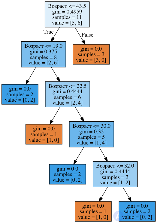
In the figure below we see that the tree used 5 values against which age is compared: 43.5, 19, 22.5, 30, and 32 years. If you look closely, these are exactly the average values between the ages at which the target class "changes" from 1 to 0 or vice versa. This is a complicated phrase, so here's an example: 43.5 is the average between 38 and 49 years, a client who is 38 did not repay the loan, while one who is 49 did repay it. Similarly, 19 years is the average between 18 and 20 years. That is, as thresholds for "cutting" a quantitative feature, the tree "looks" at those values at which the target class changes its value.
Think about why it doesn't make sense in this case to consider the feature "Age < 17.5".
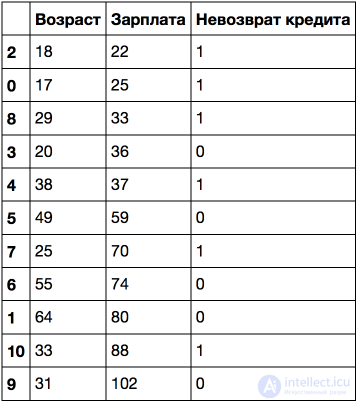
Let's consider a somewhat more complex example: let's add the feature "Salary" (thousand rubles/month).
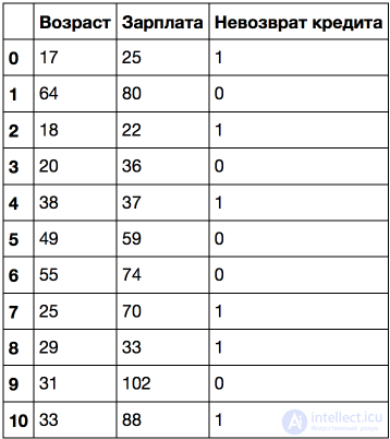
If sorted by age, the target class ("Loan default") changes (from 1 to 0 or vice versa) 5 times. And if sorted by salary – 7 times. How will the tree choose features now? Let's see.
Code for training and plotting the tree
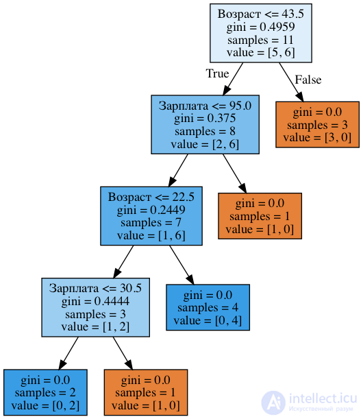
We see that the tree involves splits both by age and by salary. Moreover, the thresholds against which the features are compared are: 43.5 and 22.5 years – for age, and 95 and 30.5 thousand rubles/month – for salary. And again we can notice that 95 thousand is the average between 88 and 102, and a person with a salary of 88 turned out to be "bad", while one with 102 – "good". The same goes for 30.5 thousand. That is, comparisons of salary and age were not tried against all possible values, but only against a few. And why did these particular features end up in the tree? Because splitting by them turned out better (according to the Gini impurity criterion).
Conclusion: the simplest heuristic for handling quantitative features in a decision tree is: the quantitative feature is sorted in increasing order, and only those thresholds at which the target feature changes value are checked in the tree. This doesn't sound very rigorous, but I hope I've conveyed the idea using toy examples.
Additionally, when the data has many quantitative features, and each of them has many unique values, not all of the thresholds described above may be selected, but only the top N that give the maximum gain of that same criterion. That is, essentially, for each threshold a tree of depth 1 is built, it is calculated how much the entropy (or Gini impurity) decreased, and only the best thresholds are chosen against which to compare the quantitative feature.
To illustrate: when splitting by the feature "Salary ≤ 34.5", in the left subgroup the entropy is 0 (all clients are "bad"), while in the right – 0.954 (3 "bad" and 5 "good", you can check this yourself, part 1 of the homework assignment will be exactly about getting a thorough understanding of building trees). The information gain turns out to be about 0.3.
And when splitting by the feature "Salary ≤ 95", in the left subgroup the entropy is 0.97 (6 "bad" and 4 "good"), while in the right – 0 (just one object). The information gain turns out to be about 0.11.
Having calculated the information gain for each split in this way, one can, before building a large tree (over all features), pre-select the thresholds against which each quantitative feature will be compared.
More examples of discretizing quantitative features can be found in posts like this one or this one. One of the most well-known research papers on this topic is "On the handling of continuous-valued attributes in decision tree generation" (U.M. Fayyad, K.B. Irani, "Machine Learning", 1992).
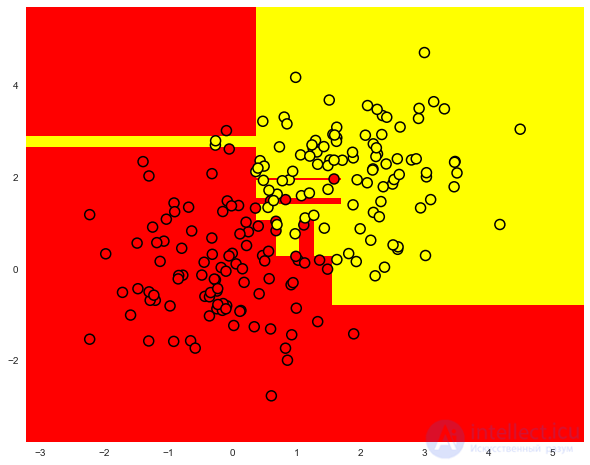
In principle, a decision tree can be built to such a depth that each leaf contains exactly one object. But in practice this is not done (if only a single tree is being built), because such a tree would be overfitted – it would fit itself too closely to the training sample and would perform poorly at predicting on new data. Somewhere down in the tree, at a great depth, splits by less important features would start to appear (for example, whether the client came from Saratov or Kostroma). To exaggerate, it might turn out that out of all 4 clients who came to the bank for a loan wearing green pants, none of them repaid the loan. But we don't want our classification model to generate such overly specific rules.
There are two exceptions, situations when trees are built to maximum depth:
The figure below is an example of a separating boundary built by an overfitted tree.
The main ways to combat overfitting in the case of decision trees:
The main parameters of the sklearn.tree.DecisionTreeClassifier class:
The tree's parameters need to be tuned depending on the input data, and this is usually done using cross-validation, which we'll cover shortly.
When predicting a quantitative feature, the idea of building the tree stays the same, but the quality criterion changes:
Example
Let's generate data distributed around the function f(x)=e−x2+1.5∗e−(x−2)2 with some noise, train a decision tree on it, and plot the predictions the tree makes.
Code
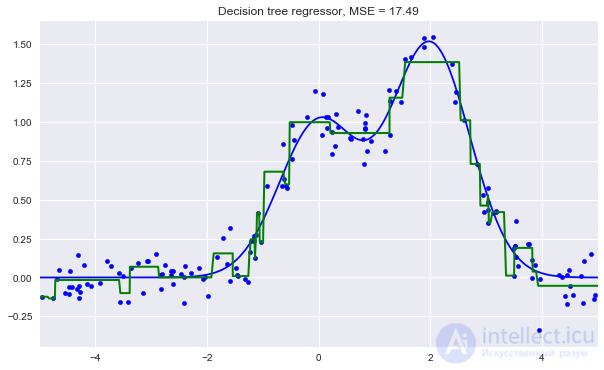
We can see that the decision tree approximates the dependency in the data with a piecewise-constant function.
The nearest neighbors method (k Nearest Neighbors, or kNN) — is also a very popular classification method, sometimes also used in regression tasks. Along with the decision tree, it is one of the most intuitive approaches to classification. On an intuitive level, the essence of the method is this: look at your neighbors, whichever type predominates, that's what you are. Formally, the method is based on the compactness hypothesis: if the distance metric between examples is chosen well enough, similar examples are much more likely to belong to the same class than to different ones.
According to the nearest neighbors method, the test example (the green ball) will be assigned to the "blue" class rather than the "red" class.
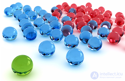
For example, if you don't know which product type to specify in a listing for a Bluetooth headset, you can find 5 similar headsets, and if 4 of them are assigned to the "Accessories" category and only one — to the "Electronics" category, then common sense suggests specifying the "Accessories" category for your listing as well.
To classify each object in the test set, the following operations must be performed in sequence:
The method can be adapted to a regression task fairly easily – at step 3, instead of a label, a number is returned – the mean (or median) value of the target feature among the neighbors.
A notable property of this approach is its laziness. This means that the computations only begin at the moment a test example is classified, and beforehand, once training examples are available, no model is built at all. This is a difference from, for example, the previously discussed decision tree, where a tree is first built based on the training set, and then classification of test examples happens relatively quickly.
It is worth noting that the nearest neighbors method is a well-studied approach (in machine learning, econometrics, and statistics, probably only linear regression is better known). For the nearest neighbors method there are quite a few important theorems stating that on "infinite" samples it is the optimal classification method. The authors of the classic book "The Elements of Statistical Learning" consider kNN to be a theoretically ideal algorithm, whose applicability is simply limited by computational capabilities and the curse of dimensionality.
The quality of classification/regression using the nearest neighbors method depends on several parameters:
The main parameters of the sklearn.neighbors.KNeighborsClassifier class:
The main task of trainable algorithms is their ability to generalize, that is, to work well on new data. Since we cannot immediately check the quality of the built model on new data (after all, we need to make predictions for it, meaning we don't know the true values of the target feature for it), we have to sacrifice a small portion of the data in order to check the model's quality on it.
Most often this is done in one of 2 ways:
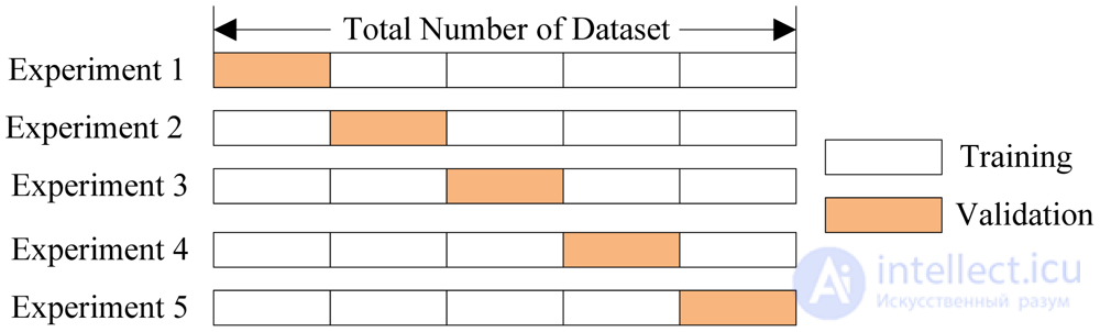
Here the model is trained K times on different (K−1) subsamples of the original set (white color), and validated on one subsample (a different one each time, orange color).
This produces K estimates of the model's quality, which are usually averaged to give the mean estimate of classification/regression quality under cross-validation.
Cross-validation gives a better estimate of the model's quality on new data compared to a held-out set. But cross-validation is computationally expensive if there is a lot of data.
Cross-validation is a very important technique in machine learning (also used in statistics and econometrics); it is used to choose model hyperparameters, compare models against each other, assess the usefulness of new features for a task, and so on. You can read more about this, for example, here from Sebastian Raschka or in any classic textbook on machine (statistical) learning
Let's read the data into a DataFrame and perform preprocessing. We'll save the states for now into a separate Series object, but remove them from the dataframe. We'll train the first model without the states, and later see whether they help.
Reading and preprocessing the data
df = pd.read_csv('../../data/telecom_churn.csv')

df['International plan'] = pd.factorize(df['International plan'])
df['Voice mail plan'] = pd.factorize(df['Voice mail plan'])
df['Churn'] = df['Churn'].astype('int')
states = df['State']
y = df['Churn']
df.drop(['State', 'Churn'], axis=1, inplace=True)

Let's set aside 70% of the set (X_train, y_train) for training and 30% will be a held-out set (X_holdout, y_holdout). The held-out set will not take part in the model parameter tuning at all; on it, at the end, after this tuning, we'll evaluate the quality of the resulting model. Let's train 2 models – a decision tree and kNN; we don't yet know which parameters are good, so at random: we take a tree depth of 5, and the number of nearest neighbors – 10.
Code
from sklearn.model_selection import train_test_split, StratifiedKFold
from sklearn.neighbors import KNeighborsClassifier

X_train, X_holdout, y_train, y_holdout = train_test_split(df.values, y, test_size=0.3,
random_state=17)

tree = DecisionTreeClassifier(max_depth=5, random_state=17)
knn = KNeighborsClassifier(n_neighbors=10)

tree.fit(X_train, y_train)
knn.fit(X_train, y_train)
We'll check the quality of the predictions using a simple metric – the fraction of correct answers. Let's make predictions for the held-out set. The decision tree did better: the fraction of correct answers is about 94% versus 88% for kNN. But so far we've been choosing the parameters at random.
Code for evaluating the models
from sklearn.metrics import accuracy_score

tree_pred = tree.predict(X_holdout)
accuracy_score(y_holdout, tree_pred) # 0.94
knn_pred = knn.predict(X_holdout)
accuracy_score(y_holdout, knn_pred) # 0.88
Now let's tune the tree's parameters using cross-validation. We'll tune the maximum depth and the maximum number of features used at each split. The essence of how GridSearchCV works: for each unique pair of values of the max_depth and max_features parameters, 5-fold cross-validation will be performed, and the best combination of parameters will be selected.
Tuning the model parameters
from sklearn.model_selection import GridSearchCV, cross_val_score
tree_params = {'max_depth': range(1,11),
'max_features': range(4,19)}
tree_grid = GridSearchCV(tree, tree_params,
cv=5, n_jobs=-1,
verbose=True)
tree_grid.fit(X_train, y_train)
The best combination of parameters and the corresponding mean fraction of correct answers under cross-validation:
tree_grid.best_params_
{'max_depth': 6, 'max_features': 17}
tree_grid.best_score_
0.94256322331761677
accuracy_score(y_holdout, tree_grid.predict(X_holdout))
0.94599999999999995
Now let's try tuning the number of neighbors in the kNN algorithm.
from sklearn.pipeline import Pipeline
from sklearn.preprocessing import StandardScaler
knn_pipe = Pipeline([('scaler', StandardScaler()), ('knn', KNeighborsClassifier(n_jobs=-1))])
knn_params = {'knn__n_neighbors': range(1, 10)}
knn_grid = GridSearchCV(knn_pipe, knn_params,
cv=5, n_jobs=-1,
verbose=True)
knn_grid.fit(X_train, y_train)
knn_grid.best_params_, knn_grid.best_score_
({'knn__n_neighbors': 7}, 0.88598371195885128)
accuracy_score(y_holdout, knn_grid.predict(X_holdout))
0.89000000000000001
In this example, the tree performed better than the nearest neighbors method: 94.2% correct answers under cross-validation and 94.6% on the held-out set versus 88.6% / 89% for kNN. Moreover, in this task the tree performs very well, and even random forest (which for now we present simply as a bunch of trees that together, for some reason, work much better than a single tree) shows a fraction of correct answers not much higher in this example (95.1% under cross-validation and 95.3% – on the held-out set), but takes much longer to train.
Code for training and tuning the random forest
from sklearn.ensemble import RandomForestClassifier

forest = RandomForestClassifier(n_estimators=100, n_jobs=-1, random_state=17)
print(np.mean(cross_val_score(forest, X_train, y_train, cv=5))) # 0.949
forest_params = {'max_depth': range(1,11),
'max_features': range(4,19)}
forest_grid = GridSearchCV(forest, forest_params,
cv=5, n_jobs=-1,
verbose=True)
forest_grid.fit(X_train, y_train)
forest_grid.best_params_, forest_grid.best_score_ # ({'max_depth': 9, 'max_features': 6}, 0.951)
accuracy_score(y_holdout, forest_grid.predict(X_holdout)) # 0.953
Let's draw the resulting tree. Since it's not exactly a toy tree (maximum depth – 6), the picture ends up not being small, but you can "take a walk" through the tree if you open the image separately.
Code for drawing the tree
export_graphviz(tree_grid.best_estimator_, feature_names=df.columns,
out_file='../../img/churn_tree.dot', filled=True)
!dot -Tpng '../../img/churn_tree.dot' -o '../../img/churn_tree.png'

Continuing the discussion of the pros and cons of the methods discussed, let's give a very simple example of a classification task that the tree handles, but in a somewhat more "complicated" way than we'd like. Let's create a set of points on a plane (2 features); each point will belong to one of the classes (+1, red, or -1 – yellow). If we look at this as a classification task, everything seems very simple – the classes are separated by a straight line.
Code for generating the data and the picture
def form_linearly_separable_data(n=500, x1_min=0, x1_max=30, x2_min=0, x2_max=30):
    data, target = [], []
    for i in range(n):
        x1, x2 = np.random.randint(x1_min, x1_max), np.random.randint(x2_min, x2_max)

        if np.abs(x1 - x2) > 0.5:
            data.append([x1, x2])
            target.append(np.sign(x1 - x2))
    return np.array(data), np.array(target)

X, y = form_linearly_separable_data()

plt.scatter(X[:, 0], X[:, 1], c=y, cmap='autumn', edgecolors='black');
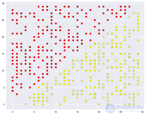
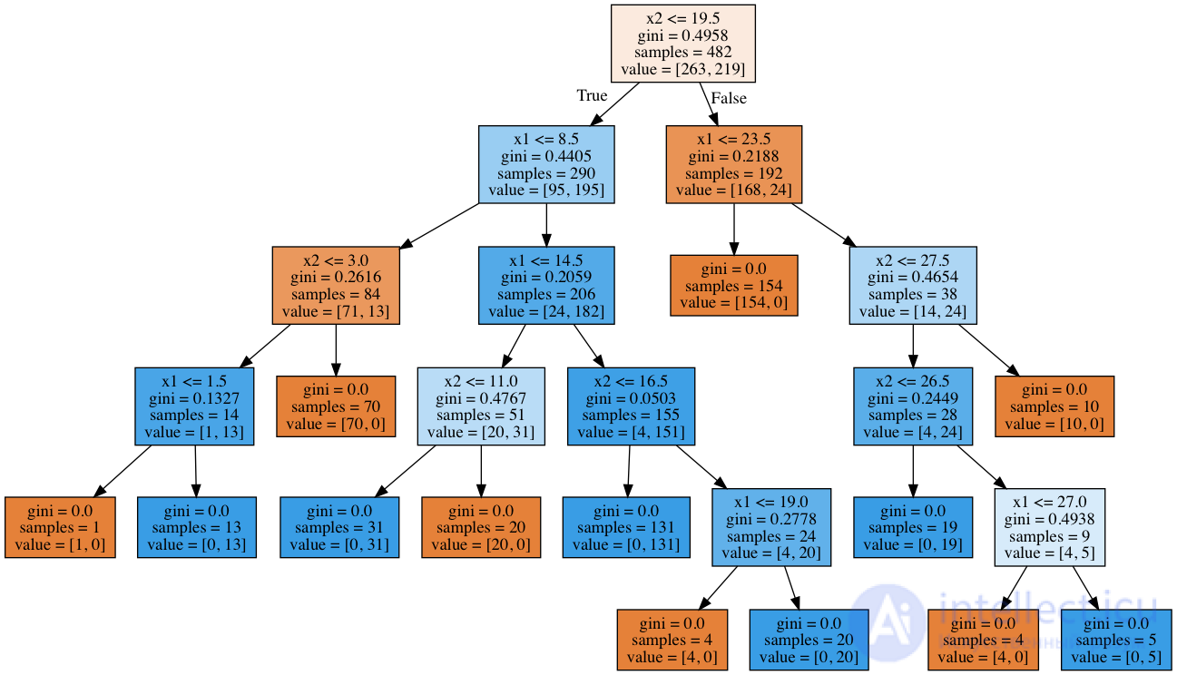
However, the decision tree builds a needlessly complex boundary and turns out to be deep on its own. Also, imagine how poorly the tree will generalize to the space outside the 30×30 square shown, which bounds the training set.
Code for drawing the separating surface built by the tree
tree = DecisionTreeClassifier(random_state=17).fit(X, y)

xx, yy = get_grid(X, eps=.05)
predicted = tree.predict(np.c_[xx.ravel(), yy.ravel()]).reshape(xx.shape)
plt.pcolormesh(xx, yy, predicted, cmap='autumn')
plt.scatter(X[:, 0], X[:, 1], c=y, s=100,
cmap='autumn', edgecolors='black', linewidth=1.5)
plt.title('Easy task. Decision tree compexifies everything');
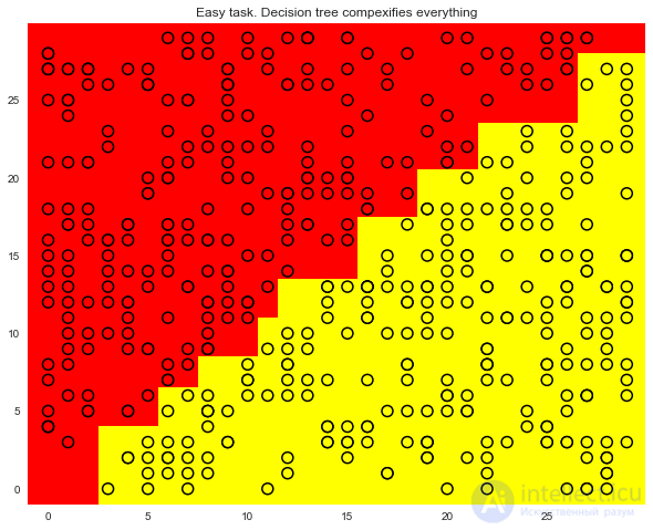
Here is such a complex construction, even though the solution (a good separating surface) is just the line x1=x2.
Code for drawing the tree
export_graphviz(tree, feature_names=['x1', 'x2'],
out_file='../../img/deep_toy_tree.dot', filled=True)
!dot -Tpng '../../img/deep_toy_tree.dot' -o '../../img/deep_toy_tree.png'
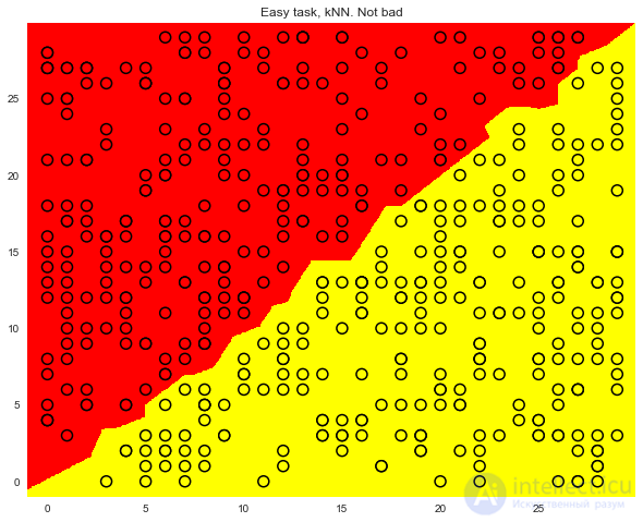
The one-nearest-neighbor method seems to handle this better than the tree, but still not as well as a linear classifier (our next topic).
Code for drawing the separating surface built by kNN
knn = KNeighborsClassifier(n_neighbors=1).fit(X, y)

xx, yy = get_grid(X, eps=.05)
predicted = knn.predict(np.c_[xx.ravel(), yy.ravel()]).reshape(xx.shape)
plt.pcolormesh(xx, yy, predicted, cmap='autumn')
plt.scatter(X[:, 0], X[:, 1], c=y, s=100,
cmap='autumn', edgecolors='black', linewidth=1.5);
plt.title('Easy task, kNN. Not bad');
Now let's look at these 2 algorithms on a real task. We'll use the handwritten digit data "built into" sklearn. This task will be an example where the nearest neighbors method works surprisingly well.
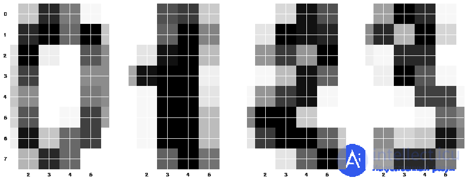
Here, images are represented as an 8 x 8 matrix (the intensity of white for each pixel). This matrix is then "unrolled" into a vector of length 64, giving the feature description of the object.
Let's draw a few handwritten digits; we can see that they are recognizable.
Loading the data and drawing a few digits
from sklearn.datasets import load_digits

data = load_digits()
X, y = data.data, data.target

X[0,:].reshape([8,8])
array([[ 0., 0., 5., 13., 9., 1., 0., 0.],
[ 0., 0., 13., 15., 10., 15., 5., 0.],
[ 0., 3., 15., 2., 0., 11., 8., 0.],
[ 0., 4., 12., 0., 0., 8., 8., 0.],
[ 0., 5., 8., 0., 0., 9., 8., 0.],
[ 0., 4., 11., 0., 1., 12., 7., 0.],
[ 0., 2., 14., 5., 10., 12., 0., 0.],
[ 0., 0., 6., 13., 10., 0., 0., 0.]])
f, axes = plt.subplots(1, 4, sharey=True, figsize=(16,6))
for i in range(4):
axes[i].imshow(X[i,:].reshape([8,8]));
Next let's run exactly the same experiment as in the previous task, only the ranges of the tuned parameters will be a bit different.
Tuning DT and kNN on the MNIST data
Let's set aside 70% of the set (X_train, y_train) for training and 30% will be a held-out set (X_holdout, y_holdout). The held-out set will not take part in the model parameter tuning at all; on it, at the end, after this tuning, we'll evaluate the quality of the resulting model.
X_train, X_holdout, y_train, y_holdout = train_test_split(X, y, test_size=0.3,
random_state=17)
Let's train a decision tree and kNN; again we're taking the parameters at random for now.
tree = DecisionTreeClassifier(max_depth=5, random_state=17)
knn = KNeighborsClassifier(n_neighbors=10)

tree.fit(X_train, y_train)
knn.fit(X_train, y_train)
Let's make predictions for the held-out set. We can see that the nearest neighbors method did much better. But so far we've been choosing the parameters at random.
tree_pred = tree.predict(X_holdout)
knn_pred = knn.predict(X_holdout)
accuracy_score(y_holdout, knn_pred), accuracy_score(y_holdout, tree_pred) # (0.97, 0.666)
Now, just as before, let's tune the model parameters using cross-validation, only taking into account that there are more features now than in the previous task — 64.
tree_params = {'max_depth': [1, 2, 3, 5, 10, 20, 25, 30, 40, 50, 64],
'max_features': [1, 2, 3, 5, 10, 20 ,30, 50, 64]}

tree_grid = GridSearchCV(tree, tree_params,
cv=5, n_jobs=-1,
verbose=True)

tree_grid.fit(X_train, y_train)
The best combination of parameters and the corresponding mean fraction of correct answers under cross-validation:
tree_grid.best_params_, tree_grid.best_score_ # ({'max_depth': 20, 'max_features': 64}, 0.844)
That's no longer 66%, but it's not 97% either. The nearest neighbors method works better on this dataset. In the case of a single nearest neighbor, cross-validation achieves almost 99% correct guesses.
np.mean(cross_val_score(KNeighborsClassifier(n_neighbors=1), X_train, y_train, cv=5)) # 0.987
Let's train a random forest on this same data; it usually performs better than the nearest neighbors method on most datasets. But right now we have an exception.
np.mean(cross_val_score(RandomForestClassifier(random_state=17), X_train, y_train, cv=5)) # 0.935
You'd be right to object that we haven't tuned the parameters of RandomForestClassifier here, but even with tuning the fraction of correct answers doesn't reach 98%, as it does for the single nearest neighbor method.
Experiment results
(Notation: CV and Holdout – the model's mean fraction of correct answers under cross-validation and on the held-out set, respectively. DT – decision tree, kNN – nearest neighbors method, RF – random forest)
| CV | Holdout | |
|---|---|---|
| DT | 0.844 | 0.838 |
| kNN | 0.987 | 0.983 |
| RF | 0.935 | 0.941 |
The conclusion from this experiment (and a general piece of advice): first check simple models on your data – a decision tree and the nearest neighbors method (and next time logistic regression will be added here); it may turn out that these alone already work well enough.
Now let's look at one more simple example. In this classification task, one of the features will simply be proportional to the vector of answers, but this won't help the nearest neighbors method.
Code for generating noisy data with a pattern
def form_noisy_data(n_obj=1000, n_feat=100,
продолжение следует...
Часть 1 3. Classification, Decision Trees and the Nearest Neighbors Method
Часть 2 Pros and cons of decision trees and the nearest neighbors

Comments