Это окончание невероятной информации про деревья решений.
...
random_seed=17):
np.seed = random_seed
y = np.random.choice([-1, 1], size=n_obj)
# the first feature is proportional to the target
x1 = 0.3 * y
# the other features are noise
x_other = np.random.random(size=[n_obj, n_feat - 1])
return np.hstack([x1.reshape([n_obj, 1]), x_other]), y
X, y = form_noisy_data()
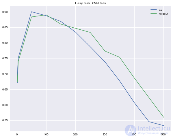
As usual, we'll look at the fraction of correct answers under cross-validation and on the held-out set. Let's build curves showing how these quantities depend on the n_neighbors parameter in the nearest neighbors method. Such curves are called validation curves.
We can see that the nearest neighbors method with the Euclidean metric can't cope with the task, even if we vary the number of nearest neighbors over a wide range. In contrast, the decision tree easily "discovers" the hidden dependency in the data for any limit on the maximum depth.
Building validation curves for kNN
from sklearn.model_selection import cross_val_score

cv_scores, holdout_scores = [], []
n_neighb = [1, 2, 3, 5] + list(range(50, 550, 50))

for k in n_neighb:

    knn = KNeighborsClassifier(n_neighbors=k)
    cv_scores.append(np.mean(cross_val_score(knn, X_train, y_train, cv=5)))
    knn.fit(X_train, y_train)
    holdout_scores.append(accuracy_score(y_holdout, knn.predict(X_holdout)))

plt.plot(n_neighb, cv_scores, label='CV')
plt.plot(n_neighb, holdout_scores, label='holdout')
plt.title('Easy task. kNN fails')
plt.legend();
Training the tree
tree = DecisionTreeClassifier(random_state=17, max_depth=1)
tree_cv_score = np.mean(cross_val_score(tree, X_train, y_train, cv=5))
tree.fit(X_train, y_train)
tree_holdout_score = accuracy_score(y_holdout, tree.predict(X_holdout))
print('Decision tree. CV: {}, holdout: {}'.format(tree_cv_score, tree_holdout_score))
Decision tree. CV: 1.0, holdout: 1.0
So, in the second example the tree handled the task perfectly, while the nearest neighbors method had trouble. However, this is a drawback not so much of the method itself as of the Euclidean metric used: in this case it failed to reveal that one feature is much better than the rest.
Pros and cons of decision trees and the nearest neighbors method
Pros and cons of decision trees
Pros:
- Generation of clear classification rules that are understandable to humans, for example, "if age < 25 and interested in motorcycles, then deny the loan". This property is called the interpretability of the model;
- Decision trees can be easily visualized, that is, both the model itself (the tree) and the prediction for an individual test object (the path through the tree) can be "interpreted" (I haven't seen a strict definition);
- Fast training and prediction processes;
- A small number of model parameters;
- Support for both numerical and categorical features.
Cons:
- Generating clear classification rules has another side to it: trees are very sensitive to noise in the input data, and the whole model can change dramatically if the training set changes slightly (for example, if one of the features is removed or a few objects are added), so the classification rules can also change a lot, which worsens the interpretability of the model;
- The separating boundary built by a decision tree has its own limitations (it consists of hyperplanes perpendicular to one of the coordinate axes), and in practice a decision tree is inferior in classification quality to some other methods;
- The need to prune the branches of the tree (pruning) or set a minimum number of elements in the tree's leaves or a maximum tree depth to combat overfitting. However, overfitting is a problem for all machine learning methods;
- Instability. Small changes in the data can substantially change the resulting decision tree. This problem is combated with ensembles of decision trees (discussed further on);
- The problem of finding the optimal decision tree (minimal in size and able to classify the set without errors) is NP-complete, so in practice heuristics are used, such as greedy search for the feature with the maximum information gain, which do not guarantee finding a globally optimal tree;
- Missing values in the data are handled with difficulty. Friedman estimated that about 50% of the code of CART (the classic algorithm for building classification and regression trees – Classification And Regression Trees; sklearn implements an improved version of precisely this algorithm) went into supporting missing values in the data;
- The model can only interpolate, not extrapolate (the same is true for forests and boosting on trees). That is, a decision tree makes a constant prediction for objects located in the feature space outside the parallelepiped that encompasses all the objects of the training set. In our example with the yellow and blue balls, this means that the model gives the same prediction for all balls with a coordinate > 19 or < 0.
Pros and cons of the nearest neighbors method
Pros:
- Simple implementation;
- Fairly well studied theoretically;
- As a rule, the method is good as a first solution to a task, and not only for classification or regression, but also, for example, for recommendation;
- It can be adapted to the task at hand by choosing the metric or kernel (in a nutshell: a kernel can define a similarity operation for complex objects such as graphs, while the kNN approach itself stays the same). By the way, Alexander Dyakonov, a professor at the CMC faculty of Moscow State University and an experienced data analysis competition participant, likes the simplest kNN, but with a tuned similarity metric for objects. You can read about some of his solutions (in particular, the "VideoLectures.Net Recommender System Challenge") on his personal website;
- A fairly good interpretation is possible; you can explain why a test example was classified in a particular way. Though this argument can be challenged: if the number of neighbors is large, the interpretation gets worse (roughly: "we denied him the loan because he is similar to 350 clients, 70 of whom are bad, which is 12% more than the average across the sample").
Cons:
- The method is considered fast compared to, for example, compositions of algorithms, but in real tasks, as a rule, the number of neighbors used for classification will be large (100-150), and in that case the algorithm will not work as fast as a decision tree;
- If a dataset has many features, it is hard to choose suitable weights and determine which features are not important for classification/regression;
- Dependence on the chosen distance metric between examples. The default choice of Euclidean distance is most often not justified by anything. A good solution can be found by trying out parameters, but for a large dataset this takes a lot of time;
- There is no theoretical basis for choosing a specific number of neighbors — only trial and error (though, admittedly, this is usually true for all hyperparameters of all models). With a small number of neighbors, the method is sensitive to outliers, that is, prone to overfitting;
- As a rule, it works poorly when there are many features, because of the "curse of dimensionality". This is described well by Pedro Domingos, a professor well known in the ML community – here, in the popular article "A Few Useful Things to Know about Machine Learning"; "the curse of dimensionality" is also described in the book Deep Learning, in the "Machine Learning basics" chapter.
With this we are coming to the end; we hope this article will last you a good while. On top of that, there is also homework.
Assignment
Current homework assignments are announced during the course's next session; you can follow them in the VK group and in the course repository.
To reinforce the material, we suggest completing this assignment – figure out how a decision tree works on a toy example, then train and tune trees for the classification task on the Adult dataset from the UCI repository. You can check yourself by submitting your answers via the web form (you'll also find the solution there).
See also
- [[b4294]]
- Nearest centroid classifier
- Closest pair of points problem
- decision theory
Продолжение:
Часть 1 3. Classification, Decision Trees and the Nearest Neighbors Method
Часть 2 Pros and cons of decision trees and the nearest neighbors
See also


Comments