
Lecture
One of the key elements of singularity theory is the notion of the multiplicity of a function or map at a point.
We shall now define it in the simplest case, for functions of one variable. The general notion of multiplicity will be introduced in Section 7.
the multiplicity of a function at a root and the multiplicity of a critical point are different notions, although both are related to the analysis of the behavior of a function.
| Notion | What it means | Where it is applied |
|---|---|---|
| Multiplicity of a root | How many times a root is repeated in the expression of the function f(x)=(x−a)k⋅g(x) | In the analysis of the zeros of a function
|
| Multiplicity of a critical point | How many consecutive derivatives vanish at the point x=a, before a nonzero derivative appears |
In the analysis of extrema and the shape of the graph
|
Let  be a smooth function and 0 its critical point, i.e. f'(0) = 0. The multiplicity of the function f(x) at the point 0 is called the order of the zero of the function f(x)−f(0), i.e. the order of tangency of the graphs y = f(x) and y = f(0).
This is a natural number µ, defined by the condition

In the case µ = 1 the critical point is called «nondegenerate» (it is clear that this agrees with the definition of a nondegenerate point given above).
We set µ = 0 for noncritical points.
If, on the other hand, no natural number µ satisfying condition (2.1) exists (i.e. the derivatives of all orders vanish at the point 0), then we set µ = ∞. In this case the function f(x) − f(0) is called «infinitely flat» at the point 0.
Critical points of infinite multiplicity can occur not only for constant functions; the reader is invited to recall the calculus course (for example, the textbook [22]) or to produce such examples independently.
In what follows we shall deal mainly with points of finite multiplicity.
The fact that in these definitions we took the origin as the point under consideration plays no role, and all the definitions carry over unchanged to the case of an arbitrary point.
PROBLEM 2.1. Compute the multiplicity of the function

at the point x = 0, given that among the coefficients of the polynomial P(x) some may be zero (including an), but they are not all simultaneously zero.
Let  be a smooth function of m + 1 variables.
We shall regard  as playing the role of the «principal variable» and
  — as the «parameters».
Fixing the value y = 0, we obtain a function f(x) of one variable, for which the notion of multiplicity was defined above.
The multiplicity µ of the function f(x) at the point 0 is called the multiplicity of the function F(x, y) with respect to the variable x at 0; it is defined by the following condition:

It is easy to see that, writing the representation (1.5) with the number p = µ + 1 , we shall have fi(0) = 0 for all i and b 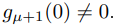 .
.
REMARK 2.1. Some authors use different terminology: if condition (2.2) holds, then the function F(x, y) is said to be (n + 1)-regular at the point 0 with respect to the variable x.

Comments