
Lecture
Take a smooth regular curve C in three-dimensional space and project it onto one of the coordinate planes along the coordinate axis perpendicular to it. In other words, we consider the restriction to the curve C of the affine map π : ®3 → R2, consisting
in «forgetting» one coordinate of that space.
Denote this restricted map by πC.
At every point of the preimage space the map π has a one-dimensional kernel — the direction of the axis along which the projection is performed'. The map πC : C → R2 has critical points precisely
where the curve C is tangent to the kernel of the projection π, see fig. 6.2 (center). The image of the map πC, the curve π(C) of the form (6.1), may have
critical points of type (6.5) with any n, m, but most often these are cusps.
The appearance of cusps can be observed in everyday life. For example, they can appear on the shadows of objects with smooth
contours. Cusps can also be observed on so-called caustics — envelopes of families of rays. Recall that the envelope (English:
envelope) of an arbitrary family of curves in the plane is
such a curve that at each of its points is tangent to one curve of that
family, but does not coincide identically with it in any
neighborhood.
Thus, for example, caustics with cusps can be observed as bright curves arising upon reflection/refraction of light rays, for example when passing through a transparent glass of water, see
fig. 6.2 (right) and fig. 6.8.
1 Formally it would be more correct here to speak of the kernel of the differential of the map π, rather than of the map itself, but since this map is affine, we allow
ourselves this liberty of speech.
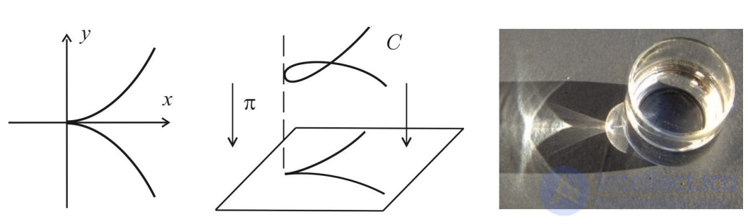
Fig. 6.2 The semicubical parabola and cusps. The curve C in the center has no
self-intersection; only its projection onto the retina of an observer looking «from the side» does
Cusps can also arise in the mechanical motion of bodies. For example, on the curve traced by a fixed point of a wheel of radius r, rolling without slipping along some smooth
surface S. For visualization, one can imagine that this point on the
wheel carries a bright mark. The curve traced by this mark has singularities at those points where the mark touches the surface S.
The reason for the appearance of singularities here is fairly obvious: in the
absence of slipping the instantaneous velocity of the «mark» at the point of contact with the surface S is zero (in mechanics such a point is called the «instantaneous center of velocities»), and hence at such
points condition (6.2) holds, and the curve of the form
(6.1) traced by the mark has a singularity. A simple argument (which we leave to the reader) shows that this singularity is a cusp.
If a wheel of radius r rolls along a straight line in the plane, the mark traces a periodic curve (with period 2πr) called a cycloid (the reader is invited to draw a cycloid on their own).
If a wheel of radius r rolls along the inside of a circle of radius R > r, the corresponding curve is called a hypocycloid. The precise shape of the hypocycloid depends on the ratio of the radii
k = R/r. Several examples are shown in fig. 6.3. For k = 3 the hypocycloid is called a deltoid, for k = 4 — an astroid. Many
pictures and even animations on this subject can be found on the Internet.
PROBLEM 6.8. Show that the hypocycloid is non-closed
if the number k is irrational, in which case it contains an infinite number of
cusps. If the number k is rational, the hypocycloid is closed and the number of
its cusps equals p, where k = p/q, with p, q integers, relatively prime.
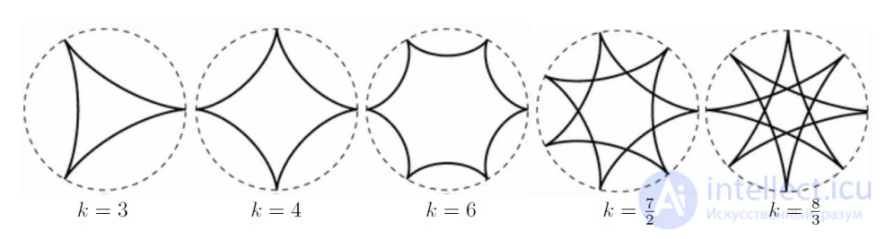
Fig. 6.3 Hypocycloids (bold lines) for various values of k
Consider real cubic polynomials
P(t) = t3 + at + b
with real coefficients a, b. Each such polynomial
can be identified with a point of the plane with Cartesian coordinates (a, b). What does the locus of points look like that correspond to
polynomials P(t) having a multiple real root?
To answer this question one must write down the equalities expressing
the presence of a multiple root: P(t) = 0 and P’(t) = 0. Regarding these
as equations in the variables a, b with parameter t, we obtain
the expressions
a = -3t2, b = 2t3,
showing that this is a semicubical parabola with a cusp at the point
a = b = 0, which corresponds to the unique polynomial with a root
of multiplicity 3.
PROBLEM 6.9. Investigate the analogous question for polynomials
P(t) = tn + at + b of arbitrary degree n > 3.
Suppose that in some continuous medium a disturbance propagates — a «wave». Assume that at the initial moment of time the
disturbance was present on some curve S0 (if the medium is a plane)
or surface (if the medium is three-dimensional space), and that the speed
of its propagation is constant and equal to 1. To find out where the
disturbance will be after time t, one must lay off along every normal to
1 For example, a shock wave, sound, light, or an epidemic. The simplest example is circles on water from a thrown stone, or a tsunami.
70
the curve (respectively, surface) S0 a vector of length t. For each fixed t one obtains a certain curve (respectively,
surface) St, consisting of the endpoints of these vectors.
The family St for all t (note that t can be not only
positive but also negative, since the normal vector can be
laid off in either of two directions) is called the wave front of the original
curve (surface) S0, see fig. 6.4 (left). The curves (surfaces)
of one family St are called parallel to S0 and to each other. This is a
natural generalization of the notion of parallel lines and planes.
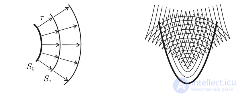
Fig. 6.4 Left: formation of a wave front. Right: the wave front
of the parabola y = x2. The bold line is the initial curve S0
It turns out that even if the original curve or surface S0 is
smooth, after some time t the wave front St may have
singularities. Let us consider, for example, the wave front St generated by the parabola y = x2 in the plane (x, y). A simple computation shows (check it!) that it is given by the formula
x = x0 − t·2x0/√(1+4x0²), y = x0² + t/√(1+4x0²) (6.13)
where x0 is the «internal» parameter on the curve. Obviously, if one lays off the normal vectors into the region y < x2 (which is equivalent to the condition t < 0), then the wave front St has no singularities at all.
If, however, one lays off the normal vectors into the region y > x2 (which
is equivalent to the condition t > 0), then, as follows from formula (6.13), for
0 < t < 1/2 the wave front St has no singularities and resembles
the original parabola S0. When the value t = 1/2 is reached, a critical point appears on St at x0 = 0. The germ of the curve St at the point x0 = 0
has the form (6.6) with exponent n = 3 and still looks fairly
smooth. Further, for every value t > 1/2 the curve St has two cusps,
located symmetrically with respect to the y-axis and moving apart from each
other as t grows; see fig. 6.4 (right).
71
PROBLEM 6.10. Draw the wave fronts generated by the curves y = xp with integer exponents p > 3 and by an ellipse, and determine
the types of their critical points.
Let C be a plane curve given in parametric form
(6.1). At every regular point of this curve its curvature
k ≥ 0 is defined, and under the additional condition k ≠ 0 the so-called osculating circle is also defined — the circle that best
approximates the curve in a neighborhood of the given point (just as
the tangent line is the line that best approximates the curve).
This is the circle of radius 1/k having a common tangent with the curve
C at the point in question and the same convexity as C. The center and
radius of the osculating circle are called the center of curvature
and the radius of curvature of the curve C at the given point.
A vertex of a curve C of the form (6.1) is a point at which the derivative of the function k(t) vanishes. A vertex is called simple
(or nondegenerate) if the second derivative of the function k(t) does not vanish at it. Thus, simple vertices are exactly the points of maximum or minimum curvature. Check question: what are the vertices
of the ellipse, the hyperbola, the parabola?
The evolute of a curve C is the locus of its centers
of curvature; we denote it E(C). This means that at every point where the curve C has a normal, a point is laid off on the normal at
distance 1/k from C, in the direction of the centripetal acceleration
arising during motion along the curve C. The evolute E(C) is also the envelope of the family of normals of the curve C (check it!).
Fig. 6.5 shows the evolutes of the parabola (left) and the ellipse
(center). These examples show that the evolute of even a smooth regular curve whose curvature vanishes nowhere may have critical points. In both examples (parabola and ellipse)
the critical points of the evolute are cusps, and they correspond to the vertices of the original curve C.
PROBLEM 6.11. Let C be a curve of the form (6.1) whose curvature
vanishes nowhere. Show that the critical points of E(C)
correspond to the vertices of C, and that the cusps of E(C) correspond to the simple vertices of C. Show that if k(t) has a critical point
of finite multiplicity q, then at the corresponding point the germ of the curve
E(C) has the form (6.6) with exponent n = q + 1. Investigate the evolute of the
graph y = xp − √(1−x2) with integer p > 2 in a neighborhood of the point x = 0.
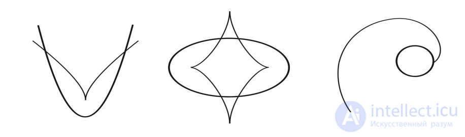
Fig. 6.5 Left: the evolute of the parabola (a semicubical parabola). Center:
the evolute of the ellipse (an astroid, four cusps). Right: the involute
of the circle referred to in Problem 6.13.
The involute of a curve C is a curve E⁻¹(C) whose evolute is C. The evolute and the involute are related to each other as the derivative and the antiderivative of a function. To one curve C there corresponds an entire
family of involutes E⁻¹(C), which are parallel to one another,
i.e. represent the wave front of one (any) of them. Thus, some involutes
in this family must necessarily
have critical points.
PROBLEM 6.12. Prove that if E(S0) = C, then E(St) = C for
any t.
For example, the evolute of the parabola y = x2 is the semicubical parabola
x = 4t3, y = t2 + 3t2 (6.14)
whose cusp is located at the focus of the original parabola (fig. 6.5, left). Let us now solve the inverse problem: find the involutes of the semicubical parabola (6.14). We already know one of its involutes: this is the parabola
y = x2. Taking the above into account, the problem reduces to finding the wave front of the parabola y = x2 — this is precisely the family of involutes.
We already know the answer, it is given by formula (6.13) and fig. 6.4 (right).
The reader is invited to check on their own that the evolute of any curve from the family (6.13) is the curve (6.14).
PROBLEM 6.13. Show that one of the involutes of the circle
x = cos t, y = sin t is the spiral x = cos t + t sin t, y = sin t − t cos t
(fig. 6.5, right). Using this, find and draw all the involutes.
PROBLEM 6.14 (*). Investigate the involutes of the cubic parabola
y = x3 and their critical points. Show that all involutes except
one have exactly two critical points: one of them is a cusp lying on the graph y = x3, and the other lies on the line y = 0 and has the form
(6.5) with exponents n = 2, m = 5.
REMARK 6.2. Evolutes and involutes have been known since ancient
times. For example, the evolutes of conic sections are discussed in the works of Apollonius of Perga³. At a more modern level, evolutes
and involutes were studied by the Dutch mathematician Christiaan Huygens in connection with his work on mechanics, in particular, on
the construction of precise mechanical clocks that would function in the presence of disturbances, for example, the pitching of a ship (the value of such an instrument for
navigation at that time is hard to overestimate)⁽. Evolutes and involutes are still used today in the gear trains of various mechanisms, for example in automobiles.
Let C be an arbitrary curve given in parametric form (6.1); its lift, or 1-graph, is the curve
C̃: x = φ(t), y = ψ(t), p = ψ’(t)/φ’(t), (6.15)
in the space J¹ with coordinates (x, y, p). Recall that J¹ is called the space of 1-jets of functions y(x).
Note that in the last equality (6.15) the denominator φ’(t) can vanish. If φ’(t) = 0 but ψ’(t) ≠ 0, then at that point
p = ∞ and the tangent to the curve C is parallel to the y-axis. One need only interchange the axes x and y, and the «division by zero» disappears. The situation is more complicated if the curve C has a nonregular point, where φ’(t) = ψ’(t) = 0.
However, in most interesting cases no problem arises here either: the function ψ’(t)/φ’(t) has a removable
singularity at the nonregular point, i.e. the left- and right-hand one-sided limits coincide, and after a suitable definition at the point itself
the function ψ’(t)/φ’(t) becomes continuous and even smooth. For example, this is the case for curves of the form (6.5) and (6.6), see fig. 6.6.
PROBLEM 6.15. Show that the result of the lift, regarded as an unparametrized curve C̃ in the space J¹, does not depend
on the choice of parametrization of the original curve C. Draw the 1-graphs
of a line, a parabola, a circle, a semicubical parabola, and a Bernoulli lemniscate (a «figure eight»).
3 An ancient Greek mathematician, one of the great geometers of Antiquity, born in the 3rd century BC in the city of Perga. He is the author of a fundamental treatise
on conic sections, in which he introduced the terms «ellipse», «hyperbola», «parabola», and many others still used throughout the world today.
4 See, for example, the popular book [8]. Some interesting properties of evolutes
and involutes, including a solution of Problem 6.14, can be found in the books [8, 35].
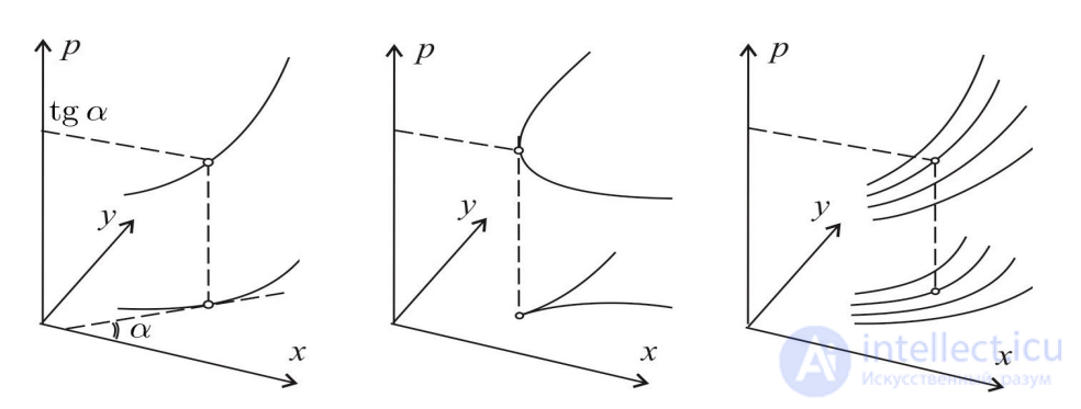
Fig. 6.6 Lift of plane curves
REMARK 6.3. The lift (English: Legendrian lift) is an important mathematical procedure. It is not hard to see that one can «lift»
not only individual curves, but also families of curves, as well as many other smooth objects. The lift occurs not only in
mathematics, but in engineering applications and even in living nature.
For example, according to current understanding in biology, the region of the primary visual cortex of the brain contains neurons organized into groups, each of which is sensitive to a particular point of the retina and a particular tangent direction at it. In this way the flat image perceived by the retina is lifted into the space of 1-jets, and the further processing performed by the brain deals with this «lifted» image.
The Legendre transform is the automorphism Λ: J¹ → J¹,
given by the formula (x, y, p) → (X, Y, P), where
X = p, P = x, Y + y = xp = XP (6.16)
The Legendre transform can be applied to various objects:
differential equations, functions, curves, and others. The objects obtained in this way are called dual to the original ones and are
often denoted by the same symbols with an asterisk. Dual
objects reflect many important properties of their preimages. The application of the Legendre transform to a curve C is expressed by the diagram
(x,y,p) —Λ→ (X,Y,P)
↓ ↓
(x,y) ——→ (X,Y)
75
where the vertical upward arrow denotes the lift of the curve C into the space J¹ with coordinates (x, y, p), the horizontal arrow «Λ» —
the automorphism Λ: J¹ → J¹, given by formula (6.16), the vertical
downward arrow — the projection π: (X, Y, P) ↦ (X, Y). As a result
of the composition of these three maps one obtains the transformation denoted by the lower horizontal arrow.
It is clear that the curve C* dual to a smooth regular curve C may have critical points: they appear under the projection π: (X, Y, P) ↦ (X, Y), as we saw in section 6.2.1.
EXAMPLE 6.2. Let us compute the dual curves for the line C1 :
y = ax + b, the parabola C2 : y = x2, and the cubic parabola C3 : y = x3.
The line can be given as x = t, y = at + b. Then p = a, and
hence X = a, Y = b, i.e. C1* is a single point.
We represent the parabola as x = t, y = t2. Then p = 2t, X = 2t, and
Y = t2. Hence C2* is the parabola Y = X2/4. We represent the cubic parabola as x = t, y = t3. Then p = 3t2, X = 3t2, Y = 2t3. Hence,
C3* is a semicubical parabola, whose cusp corresponds to the inflection point of the curve C3. The latter correspondence is by no means accidental.
PROBLEM 6.16. Show that the curve C* dual to a curve C
of the form (6.1) is regular at all points corresponding to points of the curve
C where k(t) ≠ 0, and has a cusp at points where k(t) = 0 but k’(t) ≠ 0. Consider the dual curves of the ellipse and of the fourth-degree
superellipse x4 + y4 = 1.
PROBLEM 6.17. Show that the curve C* dual to the graph C: y = f(x), where f has at the point 0 finite multiplicity n > 1,
has the form (6.6). It follows that the regular points of the curve C*
correspond to those points where f’’(x) ≠ 0, and the cusps to points of simple
(cubic) inflection: f’’(x) = 0, f’’’(x) ≠ 0. For example, fig. 6.7
shows the curve dual to the sine curve (for better visibility the scale along the x-axis is increased by about a factor of 20).
REMARK 6.4. Dual curves are also defined in other
ways. Thus, in algebraic geometry one usually uses for this purpose the transformation (x, y, p) ↦ (X, Y, P), where
X = x/y, Y = 1/y, P = dY/dX, (6.17)
the quantities X, Y being defined by formula (6.16).
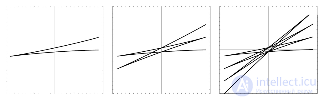
Fig. 6.7 The dual curve to y = sin x. From left to right: x ranges from 0
to 2π, 4π, 6π. The cusps of the dual curve correspond to the points x = πn
EXAMPLE 6.3. The curve dual to the ellipse (x/a)2 + (y/b)2 =1
in coordinates (X,Y) is the hyperbola Y2 − (aX)2 = b2, while in coordinates
(X, Y) it is the ellipse (aX)2 + (bY)2 = 1. There is nothing strange in the transformation of a hyperbola into an ellipse,
since the coordinates (X,Y) and (X,Y) are related
to each other by the projective transformation (6.17), and all conic
sections (which include the ellipse and the hyperbola) are projectively equivalent.
PROBLEM 6.18. Prove that the Legendre transform Λ has the property of involutivity, i.e. Λ2 is the identity map, which is equivalent to Λ = Λ⁻¹. It follows that the identity (C*)* = C
holds for any definition of duality.
If a curve C has the form of a graph y = f(x) and the curve C* dual to it
has the form of a graph Y = f*(X) for some function f*
(as we saw above, this is far from always the case — additional assumptions are needed), then the function f* is called the Legendre transform
of the original function f.
PROBLEM 6.19. Show that for the existence of the Legendre
transform of a smooth function f it suffices that the condition of strict convexity (f’’ > 0) or strict concavity (f’’ < 0) hold on the whole
domain of definition. Here the function f* is defined, generally speaking, not on the whole real line, but only on the set of values of f’.
Show that when the strict convexity condition holds, f* can
be defined by the formula
f*(p) = sup(xp − f(x)), p∈R, (6.18)
and write down its analogue for strictly concave functions.
REMARK 6.5. The Legendre transform extends
to functions of any number of variables by means of formula (6.18), where
x and p are vectors of a space of the same dimension, and xp is to be
understood as the scalar product. It is a fundamental notion of mathematics and physics, including quantum mechanics and
thermodynamics. It is difficult even to list all the possible applications
of the Legendre transform.
Perhaps its most important application is connected with the passage from the
Euler—Lagrange equations to the Hamilton equations, i.e., in the language of physics, the passage from velocities to momenta. We shall not
go into this question here, since it is treated in great detail
in many books (see, for example, [3, 21]). Instead, let us consider the
application of the Legendre transform to the example of Clairaut's equation.
The Legendre transform can be applied not only to curves,
but also to other objects of various natures. For example, consider
the first-order differential equation
F(x, y, p) = 0, p = dy/dx. (6.19)
Passing to the new variables X, Y, P by formulas (6.16) and substituting
the corresponding expressions into the left-hand side of (6.19), we obtain
a new differential equation, called dual to the original equation (6.19):
F*(X,Y,P) = 0, P = dY/dX, (6.20)
where F*(X,Y,P) = F(P, XP−Y, X).
Here only the relation P = dY/dX needs verification, and it
follows trivially from p = dy/dx and (6.16). Geometrically this means that the transformation (6.16) carries the field of planes p dx − dy = 0
into the field of planes P dX − dY = 0, or, as is often said, it preserves the contact structure of the space J¹ (the contact structure
being precisely this field of planes). From the latter property it follows
that the integral curves of the dual equation (6.20) are
dual to the integral curves of the original equation (6.19),
and conversely. This fact can be used to solve equations
explicitly, if the dual equation is simpler than the original one.
78
Let us restrict ourselves to the simplest example — Clairaut's equation:
xp − y = f(p), p = dy/dx, (6.21)
where f is an arbitrary smooth function. The Legendre transform
(6.16) turns (6.21) into the equation Y = f(X), which contains no derivative, and hence the integral curves of equation (6.21) are dual to the points
lying on the graph Y = f(X). It follows
(see Example 6.2) that the integral curves of equation (6.21) are precisely all possible lines tangent to the curve dual to the graph
of the function Y = f(X). It is not hard to see that this curve has the form
x = −f’(p), y = pf’(p) − f(p) (6.22)
and is the discriminant curve of equation (6.21) and its singular
solution (see section 13). The family of tangents to the curve (6.22)
is given by the formula y = cx − f(c) for all possible constants c,
which is obtained from equation (6.21) itself by replacing p with c.
Fig. 6.8 shows the integral curves of equation (6.21) with
function f(p) = p3. In this case curve (6.22) is the semicubical
parabola
x = −3p2; y = 2p3.
One sees that the family of nonsingular solutions — tangent lines to this
semicubical parabola — has a «thickening» near this line itself,
and especially near its cusp. This is a caustic — a line near which the intensity of the light field sharply
increases, if the tangent lines are regarded as a family of light rays. We have already seen
caustics in fig. 6.2 (right).
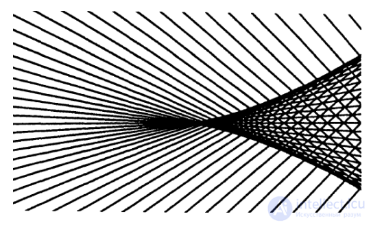
Fig. 6.8 Integral curves of Clairaut's equation xp − y = p3 — tangents
of the semicubical parabola. The figure is taken from the article [26]
One can also consider the more general equation
F(p, xp−y) = 0, p = dy/dx, (6.23)
where F(u, v) is an arbitrary smooth function. The Legendre transform turns (6.23) into F(X,Y) = 0 and, hence, the integral
curves of equation (6.23) are all possible lines tangent to the curve dual to F(X,Y) = 0. This is the discriminant curve of equation (6.23) and its singular solution; the family of tangents to it is given by the formula y = ax + b, F(a, −b) = 0.
EXAMPLE 6.4. Let us solve the equation
p3 = (xp − y)2, p = dy/dx, (6.24)
which has the form (6.23) with the function F(u,v) = u3 − v2. The dual
curve to u3 − v2 = 0 is the cubic parabola y = 2x3, which represents
the singular solution. The family of nonsingular solutions of equation (6.24)
consists of the tangents to the singular solution; they are given by the formula
y = ax + b, where a3 = b2. The latter can be rewritten as
a3 = (ax − y)2, a = const, (6.25)
or as y = c2x + c3, if we set a = c2. Formula (6.25) is obtained from equation (6.24) itself by replacing the derivative p with the constant a.
The reason for this symmetry is discussed in section 14.
The Legendre transform is not the only transformation J¹ → J¹
preserving the contact structure of the space J¹.
There is a fairly large group of transformations (by transformations we shall mean diffeomorphisms J¹ → J¹, possibly
local) that possess this property. They are called
contact or tangential transformations. An equivalent
definition: contact transformations are transformations of curves in the plane under which tangent curves are transformed into
tangent curves.
Contact transformations (x, y, p) → (X, Y, P) can be constructed
as follows:
X = F(x,y,p), Y = G(x,y,p), P = H(x,y,p),
where the functions F, G must satisfy a certain relation
(which we will now derive), and the function H is uniquely determined by them via the relation P = dY/dX. Thus, the condition for the contact structure to be preserved is the relation
dY/dX = (Gx dx + Gy dy + Gp dp)/(Fx dx + Fy dy + Fp dp) = (Gx + pGy + p’Gp)/(Fx + pFy + p’Fp) = H(x,y,p), (6.26)
where p’ = dp/dx. Since P = H(x, y, p) does not depend on p’, the expression
on the right-hand side of (6.26) must likewise not depend on p’.
The latter condition is expressed by the identity
Fp(Gx + pGy) = Gp(Fx + pFy), (6.27)
and this is precisely the relation connecting the functions F and G.
PROBLEM 6.20. Check that the Legendre transform Λ satisfies relation (6.27).
The Legendre transform is the «most important» contact transformation for applications, but historically it was not the first of them. Apparently, the first contact transformation was
the so-called pedal transformation, which is defined as follows.
Let γ be a curve in the plane and O a fixed
point, called the pole of the transformation. The pedal curve, or podary⁵,
of the curve γ with respect to the pole O is the locus
of the feet of the perpendiculars dropped from O onto all possible
tangents to the curve γ.
For example, the pedal of a circle is Pascal's snail (limaçon), the exact shape
of which is determined by the distance of the pole O from the circle (fig. 6.9).
Here we encounter a situation familiar to us: in a one-parameter family of curves a singularity arises for particular values of the parameter. Namely, when the pole O lies on the circle itself
(third picture from the left), a cusp appears on the pedal curve at the point O.
The corresponding pedal curve is called a cardioid (from
the Greek word for «heart»).
5 The name comes from the French word «pédale», which in turn comes from the word for «foot» in Greek. Podaries were first studied by Maclaurin in 1718, and later they attracted the attention of many other mathematicians, among
whom special mention should be made of Arthur Cayley and Sophus Lie. The latter is also responsible for the notion of the pedal transformation.
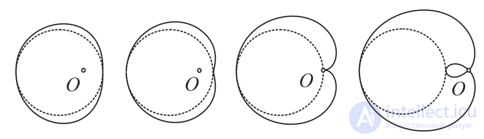
Fig. 6.9 Podaries of a circle (shown as a dotted line) — Pascal's snails
— depending on the position of the pole O
PROBLEM 6.21. Prove that if one chooses Cartesian coordinates (x,y) in the plane centered at the pole O, then the corresponding
pedal transformation is the map
P: (x, y, p) → (X, Y, P),
defined by the formulas
X = xy/(1+x2), Y = −y2/(1+x2), P = dY/dX, (6.28)
where the dependence of X, Y on x, y, p is defined in (6.16).
Note that, unlike the Legendre transform, the pedal
transformation is not an involution, so one may consider its powers (in the sense of composition) with any integer exponents. For example, let us fix the pole O as indicated in Problem 6.21,
and consider the cyclic group generated by the transformation P
with all possible integer exponents:
…, P−2, P−1, P0, P1, P2, P3, …
At first glance, it is not obvious whether this cyclic group is finite or infinite.
Sophus Lie proposed a simple and beautiful way to turn this
discrete group into a continuous one, and at the same time to prove that it is infinite. To do this, on the preimage plane with Cartesian coordinates (x, y) and on the image plane with Cartesian coordinates (X, Y)
one must introduce polar coordinates (r, φ) and (R, Φ) respectively, and
as the third coordinate of the space J¹ take the difference between the angle of inclination of the radius vector to the given point of the plane and the angle of inclination of
6 Marius Sophus Lie (1842–1899) — a Norwegian mathematician.
82
the tangent to the curve at that point, where the order of subtraction in the preimage and in the image must be opposite:
X = R cos Φ, Y = R sin Φ, x = r cos φ, y = r sin φ, (6.29)
the quantities x, y, p and X, Y, P being related by formula (6.28).
PROBLEM 6.22. Show that in coordinates (6.29) the transformation Pn with any integer n is given by the relations
R = r, Φ = p − n(p − φ), Φ = φ, (6.30)
from which, in particular, it follows that Pn ≠ Pm for any integers
n ≠ m, and hence the cyclic group {Pn} is infinite.
If in formula (6.30) n is taken not as an integer but as a real number,
one obtains no longer a discrete but a continuous group of contact
transformations. This group was first constructed by Sophus Lie.
We shall not go further into the question of contact transformations here, referring the interested reader to the specialized literature, which is quite extensive⁶.
7 See, for example: Lie S. A continuous group of contact transformations containing
as generators the pedal transformation // Tôhoku Math. J. 1940. Vol. 46. P. 252—
260. Lie S. Begründung einer Invariantentheorie der Berührungstransformationen // Math. Ann.
1875. Vol. 8. P. 215–303.

Comments