
Lecture
Let us begin with some elementary facts and notions used in singularity theory. The first will be the so-called «Hadamard’s lemma», which is surely known to many readers from the standard course in mathematical analysis (see, for example, the excellent textbook [22]). Nevertheless, we shall prove it here, in the form most convenient for further use.
Hadamard’s lemma is an important result in mathematical analysis describing the structure of a smooth function in a neighborhood of a point. It is named after the French mathematician Jacques Hadamard and is widely used in singularity theory, differential geometry, and analysis.
Consider an arbitrary smooth function
 with п >= 1 and m >= 0.
To shorten the notation we also introduce the notation  . The word «smooth», without specifying a
particular degree of smoothness, everywhere means  .
.
LEMMA 1.1 (Hadamard). The function F can be represented in the form
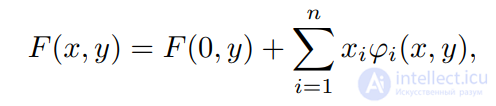 where all the
 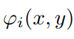 are smooth functions.
Proof. Consider the auxiliary function

where t is an additional real variable (parameter).
Let t range over the values in the interval [0, 1]; then the function F(tx, y), regarded as a function of  for each fixed value of the parameter t, traces out, in the space of smooth functions of n + m variables, a certain curve (path) with endpoints F(0, y) and F(x, y).
On the other hand, one can regard F(tx, y) as a function of the variable t, depending on the parameters  and
and  .
.
Using the second point of view, we can write the equality
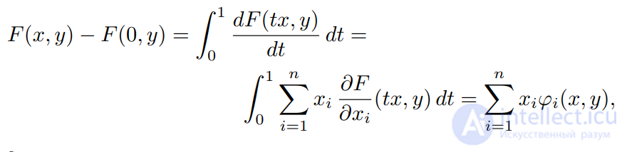 (1.2)
(1.2)
where
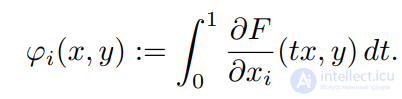 (1.3)
(1.3)
REMARK 1.1. The smoothness of the functions φi(x, y), defined by formula (1.3), follows from the well-known theorem on differentiating an integral depending on a parameter, which is proved in a course of analysis.
More precisely, from the condition F ∈ Ck, k ≥ 1, it follows that φi ∈ Ck−1. In the case under consideration,  , the required statement is obtained.
REMARK 1.2. From formula (1.1), as well as directly from (1.3), it follows that

Hadamard’s lemma is very useful for proving various facts related, in particular, to the study of singularities (critical points) of functions, mappings, etc.
PROBLEM 1.1. Prove the following generalization of Hadamard’s lemma.
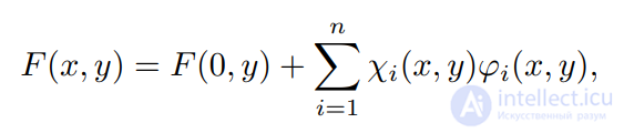
Let χ1(x, y), . . . , χn(x, y) : ВТ" - В be smooth functions, vanishing and having linearly independent gradients with respect to the variable x at the origin 0. Then, in a neighborhood of 0, the function F
can be represented in the form
 (1.4)
(1.4)
where all the φi(x, y) are smooth functions.
REMARK 1.3. Representation (1.1) is global in character, i.e., it holds for all points of the space.
It holds in the case F(x, y) :  , where X ⊂
  and
and  are domains such that X contains 0 and is convex. In contrast, representation (1.4) is local in character.
Let us consider separately the case п = 1, i.e., we shall deal with the smooth function F(x, y1, . . . , ym) : 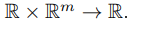 .
.
PROBLEM 1.2. Prove that for any p ∈ N a smooth function F(x, y) :  can be represented in the form
 , — (1.5)
where f1(y), . . . , fp−1(y) and gp(x, y) are smooth functions.
PROBLEM 1.3. Let F(x, y1, . . . , ym) :  be a smooth function which, in a neighborhood of the point T0 = (x0, y0), vanishes on the smooth hypersurface x = γ(y).
Then in some neighborhood of T0
the representation
 (1.6)
(1.6)
holds with a smooth function g(x, y).
PROBLEM 1.4. Let F(x, y1, . . . , ym) : be a smooth function such that, in a neighborhood of the point T0 = (x0, y0), the derivative Fx vanishes on the smooth hypersurface x = γ(y).
Then in some neighborhood of the point T0 the representation holds
 (1.7)
(1.7)
with smooth functions 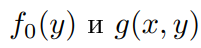 .
.
The Morse lemma: used to analyze the behavior of a function in a neighborhood of a nondegenerate critical point.
The straightening theorem for integral curves: allows one to locally bring a system of differential equations to a simple form.
Representation of the zeros of a function: if a smooth function vanishes on a hyperplane, then it can be represented as the product of the coordinate and another smooth function.
Decomposition of functions: simplifies proofs in the theory of singularities.
If the function F(x,y) is sufficiently smooth (usually continuous differentiability in x is assumed), then it can be decomposed as follows:
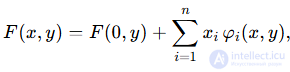
where each φi(x,y) is a smooth function.
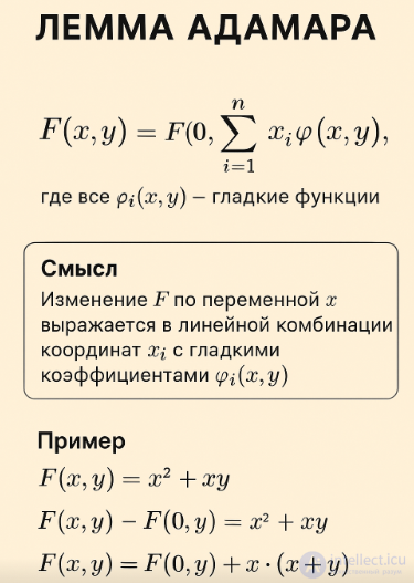
This statement says: any change in the function F(x,y) with respect to the variable x can be factored out as a linear combination of the coordinates xi, where the coefficients φi(x,y) themselves depend on (x,y) and remain smooth.
In other words, the entire dependence on x is "decomposed" over the coordinates.
Intuitively:
F(x,y) − F(0,y) is always divisible by each variable xi.
Let us take a simple function:
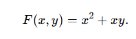
Then:
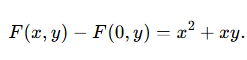
This can be rewritten as:

Here the role of  is played by (x+y).
If there were more variables, we would obtain a sum over all x.
It is a convenient technique for proofs: it allows one to decompose functions so as to work with smooth factors.
It is applied in the analysis of regularity of solutions of equations, where it is important to show that a function "behaves well" with respect to small increments.
In essence, it is a form of expansion in a neighborhood of x=0, which shows that the function is "linear in x" at the first step, with smooth coefficients.
In summary: Hadamard’s lemma says that if y is held fixed, then as x varies the function F behaves as a linear combination of the coordinates xi with smooth coefficients.

Comments