
Lecture
In mathematics, a critical point is an argument of a function at which the derivative of the function is equal to zero (or is not defined, as noted below). The value of the function at a critical point is a critical value.
More specifically, when working with functions of a real variable, a critical point is a point in the domain of the function where the derivative of the function is zero (also known as a stationary point) or where the function is not differentiable.[ Likewise, when working with complex variables, a critical point is a point in the domain of the function where its derivative is equal to zero (or the function is not holomorphic). Similarly, for a function of several real variables, a critical point is a value in its domain where the norm of the gradient is equal to zero (or is not defined).
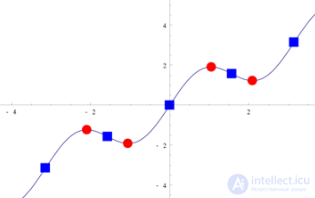
The x-coordinates of the red circles are stationary points; the blue squares are inflection points.
In mathematical analysis, a stationary point is an argument of a function at which its derivative (the gradient, for a function of several arguments) is equal to zero.
In differential calculus and differential geometry, an inflection point (a flex) is a point on a smooth plane curve at which the curvature changes sign. In particular, in the case of the graph of a function, this is a point at which the function changes from concave (downward) to convex (upward), or vice versa.
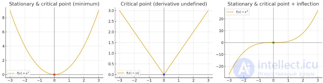
three examples in one figure:
Left: f(x)=x^2 — a stationary point and a critical point (a minimum, but not an inflection point).
Center: f(x)=∣x∣ — a critical point (no derivative exists), but not a stationary point and not an inflection point.
Right: f(x)=x^3 — a stationary point and a critical point, which is at the same time an inflection point.
Let  be a smooth function. A point x0 of the source space is called a critical point of the function F if at this point the gradient of F vanishes, i.e. all the partial derivatives
  vanish.
Critical points of functions and mappings play an important role in such areas of mathematics as differential equations, the calculus of variations, stability theory, as well as in mechanics and physics. The study of critical points of smooth mappings constitutes one of the central questions of catastrophe theory. The notion of a critical point is also generalized to the case of functionals defined on infinite-dimensional function spaces. Finding critical points of such functionals is an important part of the calculus of variations. Critical points of functionals (which are themselves functions) are called extremals.
Why are critical points interesting?
As is known from the theory of analysis, in a neighborhood of any non-critical point of a function F there exist smooth coordinates 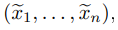 in which F becomes linear, and even takes the form

here i is any index from 1 to n.
The reader unfamiliar with this statement is invited to prove it independently, choosing as new coordinates  ;
;  ,
,
if 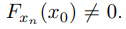 . It follows from this that in a neighborhood of a non-critical point of any smooth function, the family of level sets

is arranged in exactly the same way: it is a family of hypersurfaces in n-dimensional space which, by means of a suitable local diffeomorphism, is turned into a family of parallel hyperplanes, for example,  (see fig. 1.1 for the case of a function of two variables).
From this same argument it is evident that a function cannot attain an extremum at a non-critical point. In doing so we have incidentally proved the necessary condition for an extremum of a smooth function —
Fermat's lemma.
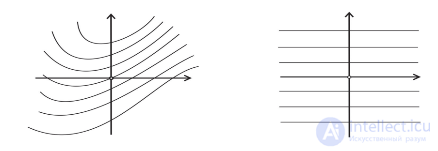
Fig. 1.1 The family of level curves of a function of two variables in a neighborhood of a non-critical point: on the left in the original coordinates, on the right in special coordinates, where this family consists of parallel lines
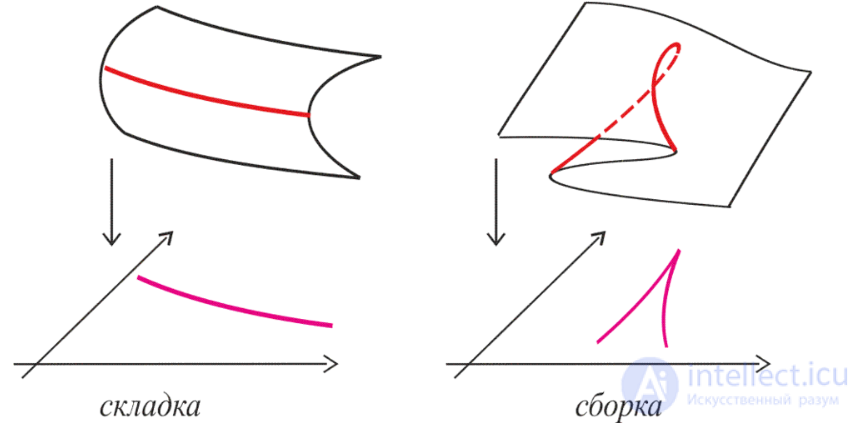
The fold and the cusp are realized as singularities of the projection of a smooth surface onto a plane.
Near critical points, the family of level sets of a smooth function may be arranged in a completely different way. To convince oneself of this, it suffices to solve the following problem.
PROBLEM 1.5. Draw the families of level curves of the following functions of two variables and verify that none of them can be carried into a family of parallel lines by means of a local diffeomorphism, and that no one of them can be carried into another:

Moreover, these families are not equivalent even topologically, i.e. they cannot be carried into one another by means of a local homeomorphism.
Thus, the problem of bringing a smooth function to a "normal" (i.e. simplest possible) form in a neighborhood of a critical point is not as trivial as in the case of a non-critical point.
Let us consider this question in more detail.
DEFINITION 1.1. A critical point  of a smooth function F(x1, . . . , xn) is called non-degenerate if the Hessian of the function F is non-zero at this point, i.e. the determinant of the matrix
 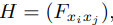 formed from the second-order partial derivatives of the function F at x0 is non-zero.
REMARK 1.4. It should be kept in mind that the term "Hessian" is sometimes used to refer not only to the determinant of the matrix H described above, but also to the matrix itself. It is usually clear from the context which of the two
is meant.
Non-degenerate critical points are the simplest type of critical point; the behavior of the function near them is completely determined by its quadratic part (recall that the linear part vanishes at a critical
point).
Namely, the following result holds:
LEMMA 1.2 (Morse's lemma). If a function  has the origin 0 as a non-degenerate critical point, then in a neighborhood of 0 there exist smooth coordinates in which the function F has the form
 . (1.8)
It is clear that an analogous representation holds in a neighborhood of any non-degenerate critical point that is not the origin. It suffices to make a shift in the space of variables carrying the point under consideration to 0, write down the representation (1.8), and then perform the inverse shift.
We shall now prove not only Morse's lemma but also a more general statement (sometimes called the "Morse lemma with parameters" or the "splitting lemma"), from which the representation
(1.8) is obtained as a particular case.
A homeomorphism is a one-to-one and bicontinuous mapping, not necessarily differentiable. Let us stress that the condition "bicontinuous" is essential: from the bijectivity and continuity of f it does not in general follow that the inverse function  is also continuous.
LEMMA 1.3 (Morse's lemma with parameters).

be a smooth function having the origin 0 as a critical point, non-degenerate with respect to the variables  .
.
Then in a neighborhood of the point 0 there exist smooth coordinates in which F has the form
 (1.9)
(1.9)
where f is some smooth function.
Proof.
We use induction on the number n. For n = 0 this statement is a tautology, and for n = 1 it is easily proved by means of problem 1.4. Indeed, for n = 1 we have a function
F(x, y), for which the derivative Fx vanishes at the point 0, while
the second derivative Fxx ≠ 0. Consequently the function Fx has 0 as a non-critical point and vanishes on some smooth
hypersurface x = τ(y) passing through 0. Using representation (1.7) and making the substitution x ↦ x − τ(y), we obtain
the representation

where  are smooth functions.
The substitution  gives
gives 
in which the number  depends on the sign of
  .
.
The induction step (for n > 1) is based on the very same idea.
One only needs to "split off" one variable from among  from all the others. Let us do this.
As is known from linear algebra, any quadratic form can be brought to canonical (diagonal) form by means of a non-degenerate linear transformation.
By hypothesis, the quadratic part of the function F with respect to the variables x1, ..., xm at the point 0 is non-degenerate, and therefore, by means of a suitable linear transformation, it can be brought to the form
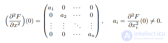
In accordance with this, let us relabel the variables and represent our function F in the form  where
where 
 . Then the partial derivative Fx1 vanishes at the point 0, while the second partial derivative
  is non-zero.
Consequently, the function Fx1 has 0 as a non-critical point and vanishes on some smooth hypersurface  passing through 0.
Using representation (1.7) and the substitution  , we obtain the representation

where  are smooth functions, and moreover
  .
.
Now making the substitution  , we obtain the equality

in which the number  depends on the sign of
  .
.
The function  depends on one fewer variable:
  .
.
Moreover, as is easily seen, 0 is a critical point of this function, non-degenerate with respect to the variables  .
.
Applying induction on n, we obtain the desired representation (1.9).
The classical "Morse lemma" is the special case m = 0.

Comments