
Lecture
Suppose we are given an equation
F(x; t) = 0;  (2.4)
(2.4)
where F is a smooth (or analytic) function and F(0; 0) = 0.
Consider the following problem: solve equation (2.4) for the variable x, i.e., find a solution of the form x = f(t), in a neighborhood of the origin 0 of the plane of variables (t; x).
If  then, by the implicit function theorem, in a neighborhood of 0 the solution is given in the form x = f(t) with a smooth (respectively, analytic) function f.
In the analytic case, the solution x = f(t) can be written as a convergent power series in the variable t.
But what will the solution x = f(t) look like if Fx(0) = 0, so that the implicit function theorem does not apply?
We shall answer this question under the assumption that 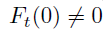 and the function F(x; t) has finite multiplicity in the variable x at the point 0, i.e., relation (2.2) holds.
From the condition  it follows that in a neighborhood of 0 equation (2.4) defines a smooth (analytic) curve of the form t = g(x).
Clearly, there are two geometrically distinct cases: if the multiplicity μ is odd, then the function g(x) has a local maximum or minimum at x = 0; if, on the other hand, the multiplicity μ is even, then the function g(x) has
an inflection point at x = 0 and is monotone on either side of it, see Fig. 2.1.
Making, if necessary, the change of variable t → -t, we shall henceforth assume that in the odd-μ case the function g(x) has a local minimum at the point х = 0, while in the even case it is increasing.
As the figure shows, in the latter case there exists a unique solution x = f(t), defined both for positive and for negative values of t, while in the first case there are two solutions of the form
x = f(t), defined only for t >= 0.
These two solutions are called the branches of the curve defined by equation (2.4), and the point x = 0 at which they meet is called the branch point of the curve.
The simplest example is the branches of the parabola t = x2.
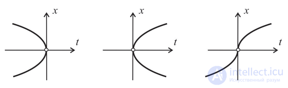
Fig. 2.1 Branch points of a curve
What will the solution (or solutions) x = f(t) look like under the assumptions made?
This question was first studied by Newton in the case where F is a polynomial. He expressed the solutions x = f(t) using power series, but not with integer, rather with fractional powers.
Later (1850) such series were studied in more detail and more systematically by the French mathematician Victor Puiseux (Victor Alexandre Puiseux, 1820-1883), in whose honor they are called «Puiseux series», and also «Newton–Puiseux series».
The division theorem allows one to obtain results analogous to those obtained by Newton, for smooth or analytic functions F.
Under the assumption made,  , it follows that in a neighborhood of 0 the equation F(x; t) = 0 is equivalent to
 (2.5)
(2.5)
where all the  are smooth (respectively, analytic) functions vanishing at t = 0.
Consequently, the аi can be represented in the form  with smooth (analytic) functions
  , and equation (2.5) can be rewritten in the form
 (2.6)
(2.6)
Let us make the substitution  and extract the root of degree
  from both sides of equation (2.6).
Here the difference between even and odd μ shows up: in the first case the root is extracted uniquely, while in the second one must affix a sign  (corresponding to the different branches of the curve).
Thus, we bring equation (2.6) to the form
 (2.7)
(2.7)
where  , if μ is even, and
  , if μ is odd.
For any fixed sign, the right-hand side of (2.7) represents, in a neighborhood of 0, a smooth (respectively, analytic) function of the variables  .
.
Applying the implicit function theorem, this equation can be locally solved for x, yielding the solution 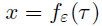 with a smooth (analytic) function
 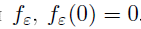 .
.
Returning to the original variable t, we obtain the solutions 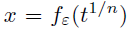 , where
 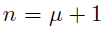 .
.
For odd n such a solution is unique and defined both for positive and for negative t.
For even n we obtain two solutions, defined for  .
.
These solutions correspond to the two branches of the curve defined by equation (2.4).
In the analytic case, the functions  can be represented as convergent (at least in some neighborhood of the point 0) power series (with integer exponents).
Consequently, the solutions 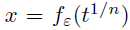 can be represented as convergent series with exponents
 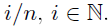 .
.
Newton–Puiseux series arise in many problems related to singularities.
Let us consider the simplest example of this kind — the curve  , given in parametric form:
 (2.8)
(2.8)
where  are smooth or analytic functions.
DEFINITION 2.1. A point of the curve (2.8), corresponding to some value of the parameter t, is called regular if at it the condition
 , (2.9)
holds, and non-regular, or singular, otherwise.
The intuitive meaning of the regularity condition (2.9) is that the curve can be parametrized in such a way (formula (2.8)) that the velocity vector of motion along the curve at the given point is nonzero.
As follows from the implicit function theorem, in a neighborhood of any regular point the curve  is the graph of a smooth (respectively, analytic) function y = f(x) or x = g(y).
If, however, we want to understand what the curve  looks like in a neighborhood of a singular point, the implicit function theorem turns out to be insufficient.
Without loss of generality we shall assume that the singular point under consideration, 0, is the origin of coordinates and  .
.
Suppose that at least one of the functions φ, ψ has finite multiplicity at zero.
Let, to be definite,  have multiplicity
  at zero, and let the multiplicity
  at zero be not less than
  .
.
Then, as is easily seen (for example, by applying Hadamard's lemma), by means of a change of parameter  with a suitable number
  (and, if necessary, a trivial change
  )
)
the curve  can be brought to the form
 (2.10)
with a smooth (respectively, analytic) function f.
From formula (2.10) one sees that the curve  has the form
 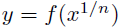 for odd n, while for even n it has two branches
  , lying in the region
  .
.
In the analytic case all these formulas give representations in the form of Newton—Puiseux series.
PROBLEM 2.2. Write down the Newton—Puiseux series for the branches of the algebraic curve x3 + ax = t, where  is a parameter, in neighborhoods of its branch points (i.e., points at which the projection of the curve onto
the t-axis is not a local diffeomorphism).
PROBLEM 2.3. Write down the Newton–Puiseux series for the branches of the function arccos t in a neighborhood of the point t = 1.
1 Weierstrass K. Einige auf die Theorie der analytischen Funktionen mehrerer Ver-anderlichen sich beziehende Satze Mathematische Werke. 1895. V. 2. P. 135-188.

Comments