
Lecture
Parallel of a curve is
It generalizes the concept of parallel lines . It can also be defined as
These two definitions are not fully equivalent, since the latter presupposes smoothness , while the first does not.
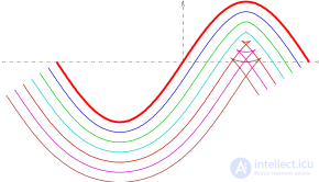
Parallel curves of the graph 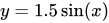 at distances
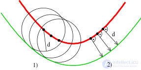
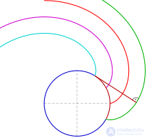
Two definitions of a parallel curve: 1) the envelope of a family of congruent circles, 2) fixed normal distance
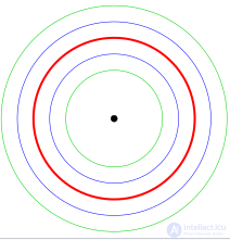
Parallel curves of a circle (red) are also circles
In computer-aided design, the preferred term for a parallel curve is offset curve . (In other geometric contexts, the term «offset» may also refer to translation . ) Offset curves are important, for example, in numerically controlled machining , where they describe, for example, the shape of a cut made. by a round cutting tool of a two-axis machine. The shape of the cut is offset from the tool path by a constant distance in a direction perpendicular to the tool path at every point.
In the field of computer 2D graphics, known as vector graphics , the (approximate) computation of parallel curves is involved in one of the fundamental drawing operations called stroking, which is usually applied to polylines or a polyline (themselves called paths) in this field.
Except in the case of a line or a circle , parallel curves have a more complex mathematical structure than the parent curve. For example, even if the parent curve is smooth , its offsets may not be; this property is illustrated in the top figure using a sinusoidal curve as the parent curve. In general, even if a curve is rational , its offsets may not be. For example, the offsets of a parabola are rational curves, but the offsets of an ellipse or hyperbola are not rational, even though these original curves themselves are rational.
This notion also extends to 3D surfaces , where it is called an offset surface . Increasing a solid's volume by a (constant) offset distance is sometimes called dilation . The opposite operation is sometimes called erosion . Offset surfaces are important in numerically controlled machining , where they describe the shape of a cut made by a ball-end mill on a three-axis machine. [10] Other cutter shapes can be modeled mathematically using general offset surfaces. [11]
If a regular parametric representation  of a given available curve exists, the second definition of a parallel curve (see above) leads to the following parametric representation of the parallel curve at distance
  :
:
 with a unit normal
  .
.
In Cartesian coordinates:
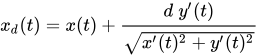
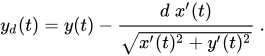
The distance parameter  can also be negative. In this case the parallel curve is obtained on the opposite side of the curve (see the diagram of parallel curves of a circle). It is easy to check: the parallel curve of a line is a parallel line in the usual sense, and the parallel curve of a circle is a concentric circle.
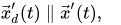 this means: the tangent vectors for a fixed parameter are parallel.
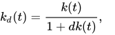 with
with  the curvature of the given curve and
 the curvature of the parallel curve for parameter
  .
. with
with  the radius of curvature of the given curve and
 the radius of curvature of the parallel curve for parameter .
If a given curve is polynomial (that is,  and
and  are polynomials), then parallel curves are generally not polynomials. In the field of CAD this is a drawback, because CAD systems use polynomials or rational curves. To obtain at least rational curves, the square root in the representation of the parallel curve must be solvable. Such curves are called Pythagorean hodograph curves and were studied by R. T. Farouki. [13]

As a rule, an analytic representation of the parallel curve of an implicit curve is not possible. Only for the simple cases of lines and circles can parallel curves be easily described. For example:
Line  → distance function:
 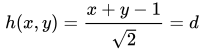 (Hesse normal form)
Circle  → distance function:
Generally speaking, assuming certain conditions, one can prove the existence of an oriented distance function  . In practice one has to treat this numerically. [14] Considering parallel curves, the following holds:
 of the corresponding oriented distance function
  .
.


Example:
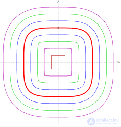
the diagram shows parallel curves of an implicit curve with equation
Note: the curves are not parallel curves, because
  does not hold true in the region of interest.
And: [16]
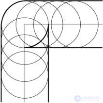
When determining the cutting path for machining a part with a sharp corner, you must determine a curve parallel to (offset from) the given curve, which has a discontinuous normal at the corner. Even if the given curve is not smooth at the sharp corner, its parallel curve can be smooth with a continuous normal, or it can have cusps where the distance from the curve coincides with the radius of curvature at the sharp corner.
As described above , the parametric representation of the parallel curve, , to a given curve,
  , at distance is:
with unit normal .
At a sharp corner ( ) the normal to
  given by
  is discontinuous, which means the one-sided limit of the normal from the left
 is not equal to the limit from the right
  . Mathematically,
 .
.
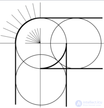
However, we can define a normal fan [11]  which provides an interpolant between and , and use in place of at the sharp corner:
 where
where  .
.
The resulting definition of the parallel curve provides the desired behavior:

An efficient compensation algorithm is the level-set approach described by Kimmel and Bruckstein (1993). [17]
For this problem there exist many approximate algorithms. For a 1997 survey, see Elber, Lee, and Kim's «Comparison of Offset Curve Approximation Methods». [18]
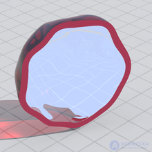
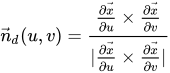
Offset surfaces are important in numerically controlled machining , where they describe the shape of a cut made by a ball-end mill of a three-axis milling machine. [10] If there exists a regular parametric representation of a given available surface, the second definition of a parallel curve (see above) generalizes to the following parametric representation of the parallel surface at distance :
 with unit normal
  .
.
The distance parameter can also be negative. In this case one obtains the parallel surface on the opposite side of the surface (see the analogous diagram of parallel curves of a circle). It is easy to check: the parallel surface of a plane is a parallel plane in the usual sense, and the parallel surface of a sphere is a concentric sphere.
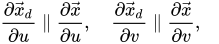 this means: the tangent vectors for fixed parameters are parallel.
 this means: the normal vectors for fixed parameters coincide in direction.
 where
where  and
and  are the shape operators for
 and
and  respectively.
The principal curvatures are the eigenvalues of this shape operator, the principal directions of curvature are its eigenvectors, the Gaussian curvature is its determinant, and the mean curvature is half its trace.
 where
where  and
and  are the inverses of the shape operators for and respectively.
The principal radii of curvature are the eigenvalues of the inverse shape operator, the principal directions of curvature are its eigenvectors, the reciprocal of the Gaussian curvature is its determinant, and the mean radius of curvature is half its trace.
Note the similarity with the geometric properties of parallel curves.
The problem quite obviously generalizes to higher dimensions, for example to offset surfaces, and somewhat less trivially to pipe surfaces. [20] Note that the terminology for the multidimensional versions varies even more widely than in the plane case, for example other authors speak of parallel fibers, ribbons and tubes. [21] For curves embedded in 3D surfaces, the offset can be produced along a geodesic. [22]
Another way to generalize this (even in 2D) is to consider a variable distance, for example parameterized by another curve. [19] One can, for example, trace (envelope) with an ellipse instead of a circle [19], as is possible, for example, in METAFONT. [23]
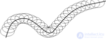
More recently Adobe Illustrator added several similar capabilities in the CS5 version, although the control points for variable width are specified visually. [24] In contexts where it is important to distinguish constant and variable distance offsetting, the abbreviations CDO and VDO are sometimes used.
Suppose you have a regular parametric representation of a curve,  , and you have a second curve, which can be parameterized by its unit normal,
  , where the normal
  (this parameterization by normal exists for curves whose curvature is strictly positive or negative and, therefore, convex, smooth and non-straight). The parametric representation of a general offset curve offset by is:
 where unit normal .
Note that the trivial offset,  , gives you the ordinary parallel (in other words, offset) curves.
this means: the tangent vectors for a fixed parameter are parallel.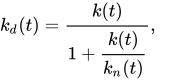 with the curvature of the general offset curve, the curvature of , and
  the curvature of
  for parameter .
 with the radius of curvature of the general offset curve, the radius of curvature of , and
  the radius of curvature of for parameter .
General offset surfaces describe the shape of the cuts made by various cutting heads used by three-axis end mills in numerically controlled machining. [11] Suppose you have a regular parametric representation of a surface,, and you have a second surface, which can be parameterized by its unit normal, , where the normal (this parameterization by normal exists for surfaces whose Gaussian curvature is strictly positive and, therefore, convex, smooth and non-flat). The parametric representation of a general offset surface offset by is:
 where
where  unit normal
  .
.
Note that the trivial offset, , gives you the ordinary parallel (in other words, offset) surfaces.
 where
where  and
and  are the shape operators for
 and respectively.
The principal curvatures are the eigenvalues of this shape operator, the principal directions of curvature are its eigenvectors, the Gaussian curvature is its determinant, and the mean curvature is half its trace.
 where
where  and
and  are the inverses of the shape operators for and respectively.
The principal radii of curvature are the eigenvalues of the inverse shape operator, the principal directions of curvature are its eigenvectors, the reciprocal of the Gaussian curvature is its determinant, and the mean radius of curvature is half its trace.
Note the similarity with the geometric properties of general offset curves.
The geometric properties listed above for general offset curves and surfaces can be derived for offsets of arbitrary dimension. Suppose you have a regular parametric representation of an n-dimensional surface, , where the dimension
  is n-1. Also suppose you have a second n-dimensional surface, which can be parameterized by its unit normal,, where the normal (this parameterization by normal exists for surfaces whose Gaussian curvature is strictly positive and, therefore, convex, smooth and non-flat). The parametric representation of a general offset surface offset by is:
 where
where  unit normal . (The trivial offset,, gives the ordinary parallel surfaces.)
First, note that the normal  normal
 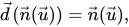 by definition. Now let us apply the differential with respect to to , which gives us its tangent vectors, spanning its tangent plane.

Note that the tangent vectors for are the sum of the tangent vectors for and its offset , which use the same unit normal. Thus, the general offset surface has a single tangent plane and normal with and  . This corresponds to the nature of envelopes.
Now let us consider the Weingarten equations for the shape operator, which can be written as . If is invertible,
 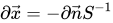 . Recall that the principal curvatures of a surface are the eigenvalues of the shape operator, the principal directions of curvature are its eigenvectors, the Gaussian curvature is its determinant, and the mean curvature is half its trace. The inverse of the shape operator preserves the same values for the radii of curvature.
Substituting into the equation for the differential , we obtained:
 where the shape operator for .
Then we again use the Weingarten equations to replace :
:
 where the shape operator for .
Then we solve for  and multiply both sides by
  to return to the Weingarten equations, this time for
 :
:


Thus,  , and inverting both sides gives us,
  .
.
Parallel curve or equidistant of a plane curve — the envelope of a family of circles of equal radius, whose centers lie on the given curve. The concept of a parallel curve — a generalization of the concept of a parallel line to the case of plane curves.
For a parametrically given curve, the parallel curve running at a distance  from the given one is defined by the equations
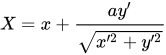 ,
,
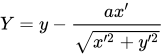 .
.
Or in vector form:

 ,
,
where the matrix  corresponds to rotating the vector 90° clockwise.
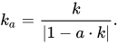
 of the parallel curve
  is expressed in terms of the curvature
  of the original curve
  by the formula
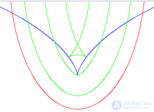
Ellipse (red), its evolute (blue) and several parallel curves (green). Note how the parallel curves break at the points where they meet the evolute

Comments