
Lecture 29 min.
The Hopfield neural network is a fully connected neural network with a symmetric matrix of connections. As such networks operate, their dynamics settle (converge) into one of the equilibrium positions. These equilibrium positions are determined in advance during training; they are local minima of a functional called the energy of the network (in the simplest case, local minima of a negative definite quadratic form on the n-dimensional cube). Such a network can be used as an autoassociative memory, as a filter, and also for solving certain optimization problems. Unlike many neural networks, which run for a definite number of steps until an answer is obtained, Hopfield networks run until equilibrium is reached, when the next state of the network is exactly equal to the previous one: the initial state is the input pattern, and at equilibrium the output pattern is obtained.
A variation of it is the Hamming neural network.
Consider a single neuron with feedback. At the first stage of operation, the input values are fed to the neuron's input and the neuron's output is computed. Then the resulting output value is fed to the neuron's input along with the other values, and a new output value is computed. This process is repeated until the neuron's output value changes only slightly from one iteration to the next.
Returning to neural networks, the following classification can be introduced. Recurrent neural networks for which it is possible to obtain outputs that stabilize at a definite value are called stable, and if the outputs of the network are not stable, then unstable. In the general case, the majority of recurrent neural networks are unstable. Unstable networks are of little use for practical applications.
In 1982 J. Hopfield proposed the architecture of a stable recurrent artificial neural network (ANN) shown in Figure 6.2. The Hopfield network has the following characteristics:
o The network is bipolar, that is, it operates only with quantities that take the values {–1, 1} or {0, 1}.
o The network has one layer of tunable neurons. Moreover, the weight matrix is symmetric.
o Each neuron is connected to all the other elements but is not connected to itself, so the main diagonal of the weight matrix contains zero elements.
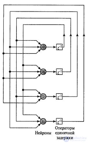
Figure 6.2 – The Hopfield network.
Initially all the patterns to be memorized xj, j = 1,...,M, are encoded as bipolar vectors of length N. These vectors are called the cells of the fundamental memory. The weights of the Hopfield network are then tuned directly from the input data on the basis of the Hebb rule:
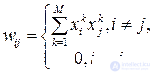 , (6.2)
where  – are the i-th and j-th components of the k-th memorized pattern.
This completes the phase in which the Hopfield network memorizes the patterns.
The matrix W has the following properties:
– it is symmetric about the main diagonal: wij = wji;
– the elements of the main diagonal are equal to zero: wii = 0;
At the beginning of the retrieval phase, the initial states of the neurons are set in accordance with the input vector – the probe. The probe may be a partially distorted pattern from the network's memory. The network then operates until the moment when it stabilizes in one of the memorized states – the attractors. The values of the outputs at that point are the recovered association. It should be noted that if the input vector is heavily distorted, the result may be incorrect.
The retrieval phase proceeds as follows. The element to be updated is chosen at random. The selected element receives the weighted signals of all the other elements and changes its state according to the following rule:
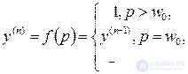 (6.3)
(6.3)
where n is the iteration number.
Another element is chosen, and the process is repeated. The network reaches its limit when none of its elements, having been selected for updating, changes its state. The elements are updated in random order, but on average each element must be updated to the same extent. For example, in the case of a network of 10 elements, after 100 updates each element should have been updated approximately 10 times.
The capacity of the network is of particular interest. In theory 2N patterns can be memorized, but in practice far fewer are obtained. It was found experimentally, and later shown theoretically, that on average, for weakly correlated patterns, a network of N neurons is able to memorize ≈ 0.15N patterns.
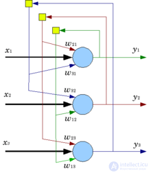
The Hopfield neural network is arranged so that its response to the memorized  reference "patterns" consists of those patterns themselves, and if a pattern is slightly distorted and fed to the input, it will be restored and the original pattern will be obtained as the response. In this way the Hopfield network performs correction of errors and noise.
The Hopfield network is single-layer and consists of  artificial neurons. Each neuron of the system can take, at its input and at its output, one of two states (which is analogous to the output of a neuron with a threshold activation function):

Because of their bipolar nature, Hopfield neural networks are sometimes called spins.
Each neuron is connected to all the remaining neurons. The interaction of the neurons of the network is described by the expression:
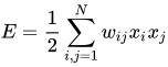
where  is an element of the interaction matrix
  , which consists of the weights of the connections between the neurons. During training an output matrix is formed, which memorizes reference "patterns" — N-dimensional binary vectors:
  ; during operation of the network these patterns will express the response of the system to the input signals, or in other words the final values of the outputs
  after a series of iterations.
In the Hopfield network the matrix of connections is symmetric ( ), and the diagonal elements of the matrix are taken to be equal to zero (
 ), which rules out the effect of a neuron acting on itself and is a necessary, but not sufficient, condition for stability during the operation of the network. A sufficient condition is the asynchronous mode of operation of the network. Properties of this kind establish a close connection with real physical substances called spin glasses.
The interaction matrix is stored on the neurons themselves in the form of the weights of the connections of the neurons with the other neurons.
So, for example, if the input signal is defined by 10 parameters, then the Hopfield neural network is formed from a single level with 10 neurons. Each neuron is connected to all the remaining 9 neurons, so that 90 (10 x 9) connections are formed in the network. A weight is defined for each connection. All the connection weights together form the interaction matrix, which is filled in during training.
Training the network consists in finding the weights of the interaction matrix in such a way as to memorize vectors (the reference patterns that make up the "memory" of the system).
The computation of the coefficients is based on the following rule: for all memorized patterns  the matrix of connections must satisfy the equation

since it is precisely under this condition that the states of the network will be stable — having entered such a state, the network will remain in it.
The vectors to be memorized must be in binary form. The weights are computed by the following formula:
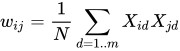
where is the dimension of the vectors, is the number of memorized output vectors,  is the index of the memorized output vector,
  is the i-th component of the memorized j-th output vector.
This expression becomes clearer if one notes that the weight matrix can be found by computing the outer product of each stored vector with itself and summing the matrices obtained in this way. This can be written as
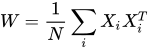
where is the i-th stored column vector.
The computation of these weights is exactly what is called training the network, and it is carried out in a single epoch only.
The Hopfield network training algorithm differs substantially from such classical perceptron training algorithms as the error-correction method or the backpropagation method. The difference is that, instead of successively approaching the required state while computing errors, all coefficients of the matrix are calculated by a single formula in one pass, after which the network is immediately ready for operation.
Some authors classify the Hopfield network as unsupervised learning. This is incorrect, however, because unsupervised learning presupposes the absence of any information about the classes to which the stimuli are to be assigned. For a Hopfield network the weights cannot be set without this information, so all that can be said here is that such a network may be assigned to the class of optimizing networks (filters). The distinctive feature of filters is that the weight matrix is set once and for all by a deterministic algorithm, and the weights are never changed afterwards. This can be convenient for the physical implementation of such a device, since at the circuit level a device with variable weights is an order of magnitude harder to build. An example of a filter without feedback connections is the CC4 (Cornel classification) algorithm, whose author is S. Kak.
A Hopfield network has feedback connections, and therefore the problem of stability has to be solved. The weights between the neurons of a Hopfield network can be regarded as an interaction matrix . Cohen and Grossberg showed that a network with feedback is stable if its matrix is symmetric and has zeros on the main diagonal. There are many stable systems of a different type — for example, all feedforward networks, as well as the modern recurrent Jordan and Elman networks, for which the symmetry condition need not be satisfied. This, however, is because other constraints are imposed on their feedback connections. In the case of a Hopfield network the symmetry condition is necessary but not sufficient, in the sense that reaching a stable state also depends on the operating mode of the network. It will be shown below that only the asynchronous mode of operation guarantees that the network reaches a stable state; in the synchronous case endless switching between two different states is possible (such a situation is called a dynamic attractor, whereas a stable state is customarily called a static attractor).
Associative memory is a distributed memory that learns on the basis of associations, much like the brain of a living creature. There are two types of associative memory: autoassociative and heteroassociative. In the autoassociative memory problem, the neural network stores the patterns (vectors) presented to it. Incomplete descriptions or noisy representations of the original patterns held in memory are then fed to this network one after another, and the task is to recognize a particular pattern. Heteroassociative memory differs from autoassociative memory in that a set of input patterns is put into correspondence with a different set of output signals.
Let xk be the key pattern (vector) used in solving the associative memory problem, and let yk be the stored pattern (vector). The pattern association relation implemented by such a network can be described as follows: yk ↔ xk, where q is the number of patterns stored in the network. The key pattern X* acts as a stimulus that not only determines the location of the stored pattern yk, but also contains the key for retrieving it.
In an autoassociative memory yk = xk. This means that the input and output data spaces of the network must have the same dimension. In a heteroassociative memory yk ≠ xk. This means that the dimension of the space of output vectors may differ from the dimension of the space of input vectors, although it may also coincide with it.
Unsupervised learning is used to tune neural networks intended for autoassociative memory problems, whereas supervised learning is used in heteroassociative memory networks.
One of the first approaches used in the unsupervised training of artificial neural networks (ANNs) is D. Hebb's rule, which in neurophysiological terms is formulated as follows:
When the axon of cell A is close enough to cell B and constantly or repeatedly takes part in firing it, a process of metabolic changes occurs in one or both neurons, as a result of which the efficiency of neuron A as one of the cells firing neuron B is increased.
As applied to artificial neural networks:
1. If two neurons on either side of a synapse are activated synchronously (that is, simultaneously), the synaptic weight of this connection increases.
2. If two neurons on either side of a synapse are activated asynchronously, this synapse is weakened or switched off altogether.
The simplest form of Hebbian learning is the following:
 (6.1)
(6.1)
where yj is the output of an element of the preceding layer and, at the same time, the input to neuron i;
wji is the weight of the input of neuron i through which the signal from neuron j is received.
A significant drawback of this implementation is that the connection strength may keep growing, which leads to unstable operation of the network. More advanced implementations are:
 – covariance learning: the deviations of the signals from their mean values over a short time interval are used;
 – differential learning: the deviations of the signal values from their values at the previous iteration are used;
 – learning with forgetting, where γ is the forgetting-rate parameter, no greater than 0.1.
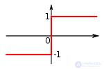
 implemented by a neuron of a Hopfield network.
As soon as the weights have been set, the trained network becomes able to "recognize" input signals — that is, to determine which of the stored patterns they belong to.
The input vector passes through a certain number of iterations until convergence is reached. Partially distorted or incomplete patterns must be recognized in the process. The values of the original vector are first applied to the input of the network (which is why showing the input synapses explicitly in the network diagram is purely a convention). The network then changes its states one after another according to the formula:

where is the activation function and and  are the current and the next states of the network; this continues until the states and coincide (or, in the case of synchronous operation, until the state
  coincides with and, at the same time,
  coincides with ). It is precisely this process that is called convergence of the network. The resulting stable state (a static attractor) or, possibly, in the synchronous case the pair {
 } (a dynamic attractor) is the network's response to the given input pattern.
The output of the network may also turn out to be the inverse vector (one in which the values -1 and 1 of the stored patterns are flipped). If the system has not found a solution, the output of the system may also be trivial vectors consisting only of 1s or only of -1s.
Since networks with feedback contain paths that carry signals from the outputs back to the inputs, the response of such networks is dynamic: after a new input is applied, the output is computed and, traveling back along the feedback connections, modifies the input. The output is then computed again, and the process repeats over and over. In a stable network, successive iterations produce ever smaller changes in the output, until the output finally becomes constant. In some networks the process never ends; such networks are called unstable. The problem of stability will be considered in the next section, while here we examine the basic cycle of the network's operation.
Once the weights have been set, the network can be used to retrieve a memorized output vector from a given input vector, which may be partly incorrect or incomplete. To do this, the outputs of the network are first assigned the values of this initial vector. The network then changes its states successively according to the formula:

where F is the activation function and  and
and  are the current and the next states of the network; this continues until the states and coincide (or, in the case of the synchronous mode of operation, until the state
  coincides with and at the same time
  coincides with ). It is precisely this process that is called convergence of the network.
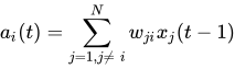
The same thing can be described by means of the so-called local field  acting on neuron
  from all the other neurons of the network:
  .
.
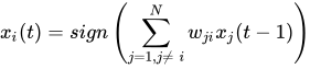
Once the local field of neuron  has been calculated, this value is used to compute the output value through the activation function, which in this case is a threshold function (with a zero threshold). Accordingly, the output value of neuron i at the current instant of time
  is calculated by the formula:
 ,
,
where is the weight between neurons i and j, and  are the output values of neuron j at the previous instant of time.
During the operation of a Hopfield network, the indication that a solution has been found is the moment at which an attractor is reached — a static one (when the stable state is repeated at every subsequent step) or, possibly, a dynamic one (when two different states {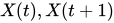 } alternate indefinitely). This final state of the network is its response to the given pattern.
A normal answer is a stable state that coincides with one of the vectors memorized during training. Under certain conditions, however (in particular, when too many patterns have been memorized), the result may turn out to be a so-called spurious attractor (a "chimera"), consisting of several fragments of different memorized patterns. In synchronous mode the network may in addition arrive at a dynamic attractor. Both of these situations are generally undesirable, since they correspond to none of the memorized vectors and therefore do not determine the class to which the network has assigned the input pattern.
Two variants of the Hopfield network are possible, differing in the signal propagation time: the asynchronous and the synchronous mode. In practice only the asynchronous mode is used.
If the operation of the network is simulated on a single processor, then in synchronous mode the neurons are scanned one after another, but their states are stored separately and are not changed until all the neurons of the network have been passed through. Once all the neurons have been scanned, their states are changed to the new ones simultaneously (that is, synchronously — hence the name). In this way the simulation of parallel operation is achieved by a sequential algorithm.
With genuinely parallel simulation, this mode in effect means that the propagation time  for every connection between elements
  and
and  is the same for all connections, which results in all the connections operating in parallel: they change their states simultaneously, relying only on the previous instant of time. It is the presence of such synchronous clock ticks, which can easily be singled out, that leads to the notion of the synchronous mode. In synchronous mode an endless alternation of two states with different energies — the so-called dynamic attractor — is possible (although it is by no means always observed). For this reason the synchronous mode is practically never used for the Hopfield network and is considered only as a basis for understanding the more complex asynchronous mode.
If the operation of the network is simulated as a sequential algorithm, then in asynchronous mode the states of the neurons at the next instant of time are changed one after another: the local field of the first neuron at instant  is computed, its response is determined, and the neuron is set to a new state (corresponding to its output at instant
  ); then the local field of the second neuron is computed taking into account the new state of the first, the state of the second neuron is changed, and so on — the state of each subsequent neuron is computed taking into account all the changes in the states of the neurons considered earlier.
In essence, in a sequential implementation of the Hopfield network it is not readily apparent where the asynchrony lies, but it becomes visible if the Hopfield network is implemented with parallel computation. In that case the asynchronous mode of the Hopfield network is simplified and constitutes a special case compared with the general form of asynchronous networks, in which the propagation time for each connection between elements and is individual but constant. In order to examine the operation of the network in a parallel implementation, it is necessary to introduce the notion of a clock tick — as the minimum time in which a signal is transmitted along a connection, that is, with  . Then a certain number N of clock ticks occurs in the interval of time between and . And it is precisely within the time of these N ticks that the asynchrony of the propagation of signals and of the execution of the computations takes place. That is, for example, when the state of neuron No. 3 has to be computed, it is necessary to compute the state of neuron No. 1 and the state of neuron No. 2 and to multiply these by the corresponding weights
  and
and  . But, as it turns out, in order to compute the state of neuron No. 2, one needs to know the updated state of neuron No. 1 and the old state of neuron No. 3, and to multiply them by the weights
  and
and  . It is clear that it is physically impossible to compute the state of neuron No. 1 and the state of neuron No. 2 at one and the same time, since the state of neuron No. 2 depends on the state of neuron No. 1. Therefore the connection between neuron No. 1 and neuron No. 3 has a propagation time
  and reaches neuron No. 3 in two clock ticks. It is precisely this difference in the propagation times that allows the Hopfield network to be spoken of as a network with an asynchronous mode.
In asynchronous mode a dynamic attractor is impossible: regardless of the number of memorized patterns and of the initial state, the network will inevitably arrive at a stable state (a static attractor).
If, during training, the matrix of weights (interneuron connections) is formed on the basis of reference binary vectors, then while the network is running it will keep changing the states of its neurons under the action of the fields described above until it settles into one of its stable states.
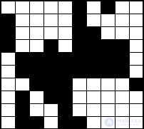
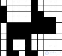
Suppose we have a neural network of dimension  , and a set of black-and-white pictures has been written into its connection matrix (−1 is black, +1 is white), among them an image of a dog (the picture on the right). If the initial state of the network is set close to this vector (the picture on the left, the distorted pattern), then in the course of its dynamics the neural network will restore the original image (the reference pattern). In this sense one may say that the Hopfield network solves the pattern recognition problem (although, strictly speaking, the reference image thus obtained still has to be converted into a class number, which in some cases can be a rather computationally demanding task).
 |
 |
| Distorted pattern | Reference pattern |
The fundamental difference between the two operating modes of the network is that in the asynchronous case the network is guaranteed to arrive at a single stable state. In the synchronous case, however, situations are possible in which it cycles endlessly between two different states.
Whether the state of a neuron is stable or not can be determined from its so-called artificial energy in the given field  . If the sign of the neuron's output (+1 or −1) coincides with the direction of the local field (
 ), then its position is energetically stable and at the next instant of time the state of the neuron remains unchanged. Otherwise (
 ) the position of the neuron is unstable and it changes its sign, passing into the state
  with energy
  .
.
Stability in the asynchronous mode is achieved because the condition on the total energy of the network  is satisfied. In the synchronous case the condition changes somewhat, namely:
  . In a situation where endless cyclic transitions occur, the energies of the two different states are, respectively,
  and
and  . Here the states and
  , as well as and
  , coincide. If such a state arises, it is called a dynamic attractor. If, on the other hand, the states and coincide, the attractor is called static. In most cases dynamic attractors are undesirable, since they do not correspond to any definite answer of the network.
A network with feedback forms an associative memory. The Hopfield network can be classified as an autoassociative memory, that is, one that can complete or correct a pattern but cannot associate the resulting pattern with another pattern. In order to organize a stable autoassociative memory by means of a network with feedback, the weights must be chosen so as to create energy minima at the required vertices of the unit hypercube.
The processing of visual patterns (filtering and associative memory) is not the only area of application of the Hopfield model. The dynamic procedure described above lowers the energy of the neural network at every step. This makes it possible to solve combinatorial optimization problems, provided they can be formulated as energy minimization problems. The classic problem of this type is the traveling salesman problem.
(The traveling salesman problem cannot be solved with a Hopfield neural network) The Hopfield network can be used to solve the traveling salesman problem (all n cities must be visited and the tour must return to the starting city in such a way that the length of the route traveled is minimal). To do this one may impose, for example, the following requirements on the network:
 neurons, which we shall regard as a square of
  rows and columns.
It turns out that the following simple considerations are sufficient to solve this problem:
 -th column must inhibit the activation of neurons in the
  -th and
  -th columns the more strongly, the greater the distance between them;
All these conditions are satisfied by the following formula for computing the weight between the neuron corresponding to city  at position in the route and the neuron corresponding to city
  at position
  :
:

where A, B, C, D are certain constants,  is the distance between cities and , and
  is the Kronecker delta, which takes the value 1 if x=y and the value 0 otherwise. As is easy to see, the first term equals
  for all connections within the same row (
 ), except for the connection of a neuron with itself (when
  ). The second term equals
  for all connections within the same column (), except for the connection with itself (). The third term is proportional to the distance between cities and if these cities are adjacent in the route (
 or
or  ).
).
If such a network is brought into a random initial state, one may expect the resulting stable state to give a suboptimal route whose length does not greatly exceed the optimal one (the route itself may differ considerably from the optimal one). Accordingly, for practical use the network should be run several times and the best route selected.
The solution of this problem is interesting not so much for its quality (there are algorithms that solve it more efficiently) as for the approach to optimization problems as such: if the conditions of some problem can be translated into the parameters of the connections between neurons, then the problem can be solved reasonably well by the network without any additional analysis.
Unfortunately, the Hopfield neural network has a number of drawbacks.
1. A relatively small memory capacity, whose magnitude can be estimated by the expression:
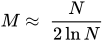
An attempt to store a larger number of patterns results in the neural network ceasing to recognize them.
2. Reaching a stable state does not guarantee a correct answer from the network. This happens because the network may converge to so-called spurious attractors, sometimes called "chimeras" (as a rule, chimeras are glued together from fragments of different patterns).

Comments