
Lecture 20 min.
Evolution is a multi-stage process in which organic forms with a higher degree of organization emerge, and it is characterized by the variability of the evolutionary mechanisms themselves. Evolutionary modeling can be defined as the reproduction of the process of natural evolution by means of special computer programs. The necessary and sufficient conditions that determine the main factors of evolution were formulated in the 20th century. The factors that make evolution inevitable are:
Figure 10.1 presents the factors of evolution in more detail, taking into account the variety of forms in which they manifest themselves, their interrelations and their mutual influence. The main factors are outlined with a dashed line.
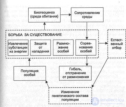
Figure 10.1 – Interrelation of the factors of evolution.
Modern evolutionary theory is based on the theory of general and population genetics. The elementary object of evolution is the population — a community of freely interbreeding individuals. Microevolutionary processes take place within populations and lead to changes in their gene pool. The genetic composition of a population is transformed under the action of elementary evolutionary factors. Random structural or functional changes in genes, chromosomes and other reproducible units are called mutations if they lead to a hereditary change in some phenotypic trait of an individual. Chromosomes are specific structures of the cell nucleus that play a crucial role in cell division. Chromosomes consist of genes. A gene is a really existing, independent unit of heredity that recombines and segregates during crossing. The gene pool of a population is transformed under the control of natural selection.
The history of evolutionary computation began with the development of a number of independent models, among which were the genetic algorithms and classifier systems created by the American researcher J. Holland. He proposed using the methods and models of the development of the organic world on Earth as a mechanism for the combinatorial enumeration of variants when solving optimization problems. Computer implementations of this mechanism came to be called "genetic algorithms".
The main directions in the development of evolutionary modeling at the present stage are the following:
It is advisable to use evolutionary methods in cases where an applied problem is difficult to formulate in a form that permits an analytical solution, or where an approximate result has to be found quickly — for example, when controlling systems in real time.
A genetic algorithm is a search algorithm based on the natural mechanisms of selection and genetics. Such algorithms ensure the survival of the fittest solutions among the many that are generated, shaping and modifying the search process by modeling the evolution of the initial population of solutions. Genetic algorithms are designed so that each new population is generated using fragments of the original solutions, to which new elements are added that improve the solutions with respect to the selection criterion that has been formulated.
Two main goals are pursued in the development of genetic algorithms:
1) an abstract and formal explanation of adaptation processes in natural systems;
2) the design of artificial software systems that reproduce the mechanisms by which natural systems function.
The main differences between a GA and other optimization algorithms:
1) not the parameters themselves but encoded sets of parameters are used;
2) the search proceeds not from a single point but from a population of points;
3) the search uses the values of the objective function rather than its increments;
4) probabilistic rather than deterministic rules of search and of solution generation are applied;
5) different regions of the solution space are analyzed simultaneously, which makes it possible to find new regions with better values of the objective function by combining quasi-optimal solutions from different populations.
Genetic algorithms are founded on genetics and on the chromosome theory of the evolution of organisms. Classical genetics accounted for heredity and variability by creating the fundamental theory of the gene, whose main propositions are formulated as follows:
1. all traits of an organism are determined by sets of genes;
2. genes are the elementary units of hereditary information, and they are located in the chromosomes;
3. genes can change — mutate;
4. mutations of individual genes lead to changes in individual elementary traits of the organism, or phenes.
Terms taken from genetics are interpreted in GAs as follows:
| Genetics | Genetic algorithms |
| Chromosome | Solution, string, line, sequence, parent, offspring |
| Population | Set of solutions (chromosomes) |
| Locus | Position of a gene in the chromosome |
| Gene | Element, characteristic, distinctive feature, property, detector |
| Generation | A cycle of operation of the genetic algorithm during which a set of solutions is generated |
| Allele | Value of an element or characteristic |
| Epistasis |
Set of parameters, alternative solutions |
Every solution among the possible ones can be represented as a body of information that can be modified by introducing into it elements of another solution. In other words, the possible solutions correspond to chromosomes made up of genes, and in the course of optimization genes are exchanged between chromosomes — recombination. Recombination is used to accumulate in the final solution the best functional traits that were present in the set of initial solutions.
Chromosomes are thread-like structures located in the cell nucleus that are the carriers of heredity. Each chromosome is morphologically and genetically unique and cannot be replaced by another one or restored if it is lost (when a chromosome is lost the cell usually dies). Every biological species has a definite, constant number of chromosomes. Each cell contains a doubled set of morphologically and genetically similar chromosomes. For example, human cells contain 23 pairs of chromosomes, and the cells of a mosquito 3.
A gene is defined as the structural unit of hereditary information that is functionally indivisible any further. The complex of genes contained in the chromosome set of a single organism forms the genome.
There are several types of recombination of chromosome segments. In genetic algorithms the most widely used is the crossing-over operation, which consists in the breakage of homologous chromatids followed by their joining in a new combination. It gives rise to a new combination of linked genes. A diagram of crossing-over, showing the formation of two new chromosomes after the exchange of genetic material, is given in Figure 10.2. The main purpose of crossing-over is to create from the available genetic material the desired combination of traits in a single solution.
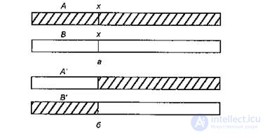
Figure 10.2 – Diagram of crossing-over:
a) parent chromosomes before crossing-over,
b) offspring chromosomes after crossing-over.
Crossing-over can occur at several points. An example of double crossing-over between chromosomes is given in Figure 10.3.
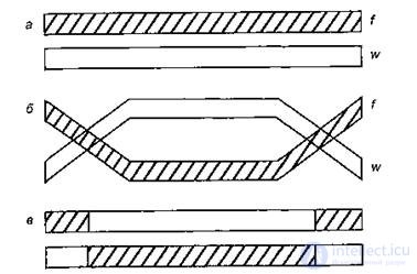
Figure 10.3 – Diagram of double crossing-over:
a) before crossing-over, b) during crossing-over,
c) after crossing-over.
Besides crossing-over, genetic operations such as mutation, inversion, translocation, selection and genetic engineering are useful for solving various applied problems.
Mutation is understood as a genetic change that leads to a qualitatively new manifestation of the basic properties of the genetic material. The use of the mutation operation in genetic algorithms is aimed at obtaining solutions that cannot be improved qualitatively by means of crossover.
Inversion, translocation, transposition, deletion and duplication are varieties of chromosomal mutation. In inversion, a segment of the chromosome is rotated through 180°. Translocation is the transfer of part of one chromosome into another. When small segments of genetic material are moved within a single chromosome, the term transposition is used. Deletion is the loss of individual chromosome segments; duplication is the repetition of a segment of genetic material. In addition to those listed, other varieties of chromosomal mutations exist.
According to Holland, genetic schemes for the search for optimal solutions include the following stages of the evolutionary process:
1. An initial population is constructed. The initial reference point for generations t = 0 is introduced. The fitness of the chromosomes of the population (the objective function) and the average fitness of the whole population are computed.
2. The value t = t+1 is set. Two parents (chromosomes) are selected for crossover. The selection is made at random in proportion to the viability of the chromosomes, which is characterized by the values of the objective function.
3. The genotype of the offspring is formed. To this end, the crossover operation is performed on the genotypes of the selected chromosomes with a given probability. One of the offspring A(t) is chosen at random, and the inversion and mutation operators are applied to it in succession with given probabilities. The resulting chromosome is stored as A’(t).
4. Updating the current population by replacing a randomly chosen chromosome with A’(t).
5. Determining the fitness of A’(t) and recomputing the average fitness of the population.
6. If t=t*, where t* is a given number of steps, then go to stage 7; otherwise go to stage 2.
7. End of operation.
The main idea of evolution embodied in the various designs of genetic algorithms manifests itself in the ability of the "best" chromosomes to exert a greater influence on the composition of the new population through longer survival and more numerous offspring.
The simple genetic algorithm includes an operation of random generation of the initial population of chromosomes and a number of operators that provide for the generation of new populations on the basis of the initial one. These operators are reproduction, crossover and mutation.
Reproduction is the process of copying chromosomes with account taken of the values of the objective function, i.e. chromosomes with "better" objective function values have a higher probability of entering the next population. This process is an analog of mitotic cell division. The selection of cells (chromosomes) for reproduction is carried out according to the principle of "survival of the fittest". The simplest way of representing the reproduction operation in algorithmic form is a roulette wheel in which each chromosome has a sector proportional to the value of the objective function.
In algorithmic implementations of the chromosome reproduction mechanism the following rules should be observed.
1. The initial population may be selected arbitrarily, for example by tossing a coin.
2. Reproduction is carried out by simulating the spin of a roulette wheel.
3. The crossover operator is implemented as a mutual exchange of short fragments of the binary strings of homologous chromosomes.
4. The probability of the crossover operator is taken equal to P(CO)<1.
5. The probability of the mutation operator is taken equal to P(MO)>0.001.
Let us consider an example of applying the simple genetic algorithm to maximize the function f(x)=x2 on the integer interval [0, 31].
The values of the function argument, which varies in the interval from 0 to 31, can be represented by five-bit binary numbers. The initial population, consisting of four five-bit numbers, was obtained by means of a random number generation procedure.
Analysis of the initial population at the first step of the simple genetic algorithm:
| Chromosome number | Value of x (decimal code) | Binary code of the chromosome | Objective function value | Selection probability | Expected number of copies of the chromosome in the next generation | Actual number of copies of the chromosome in the next generation |
| 0.14 0.49 0.06 0.31 | 0.56 1.96 0.24 1.24 | |||||
| Total | 1.00 | 4.00 | ||||
| Mean value | 0.25 | 1.00 | ||||
| Maximum value | 0.49 | 1.97 |
The probability of selecting the i-th chromosome is computed by the formula
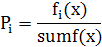
where fi(x) is the objective function value of the i-th chromosome in the population; sumf(x) is the total objective function value of all chromosomes in the population.
The expected number of copies of the i-th chromosome after the reproduction operator is equal to
N = Pin;
where n is the number of chromosomes analyzed.
Reproduction of the initial set consists in spinning the roulette wheel four times (4 is the population size), as a result of which the composition of the initial population may change.
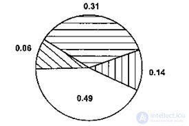
Figure 10.4 – The roulette wheel.
It should be noted that the roulette wheel does not guarantee the selection of the best chromosomes, i.e. sometimes the selection may result in chromosomes with low objective function values.
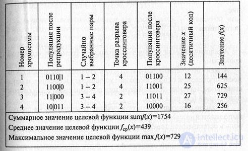
After reproduction the crossover operator is executed, and it may be repeated several times. Each time, two candidates will be selected from the set of chromosomes. Then each pair of chromosomes is crossed. The crossing point K is chosen at random in the interval (1, L-1), where L is the chromosome length, determined by the number of significant digits in its binary code. In our case L = 5. Two new chromosomes are created by mutually exchanging all values after the crossing point, i.e. between positions (K+1) and L. Selecting the first two chromosomes from the population (see the table) and the value K = 4, before applying the crossover operator we have the description:
chromosome1: 0110|1
chromosome2: 1100|0
After applying the crossover operator we obtain the description:
chromosome1: 0110|0
chromosome2: 1100|1
The offspring of the third and fourth chromosomes were obtained in the same way.
Analysis of the results obtained shows that after one generation has been carried out both the average and the maximum values of the objective function improved compared with the initial population.
According to the scheme of the simple genetic algorithm, at step 3 the mutation operator is executed, which plays an essential role in natural genetics and evolution but is less significant in genetic algorithms. Usually one mutation per 1000 bits is chosen. The mutation operator belongs to the unary operations and is implemented in two stages.
Stage 1. In the chromosome A = {a1, a2, a3…aL-2, aL-1, aL} two positions are determined at random, for example 2 and L-1.
Stage 2. The genes corresponding to the selected positions are swapped and form a new chromosome A = {a1, aL-1, a3,…, aL-2, a2, aL}
If the length of the sequences being processed is small, then in the course of mutation one can carry out an exhaustive search of the possible permutations of genes and find the combination with the maximum value of the objective function. Let us take the third chromosome 11011 with the objective function value f(x)=729 and apply the mutation operation to positions 3 and 4:
chromosome 3: 11011 -> chromosome 3': 11101.
For the new chromosome 3' the objective function value is (29)2=841. Let us make one more swap of genes 4 and 5 in chromosome 3':
chromosome 3': 11101 –> chromosome 3": 11110.
The objective function value for chromosome 3" is 900, which corresponds to a quasi-optimal solution of the problem of finding the maximum value of the function f(x)=x2 on the interval [0,31].
The Davis genetic algorithm includes the following steps:
1. Initialization of the population of chromosomes.
2. Evaluation of each chromosome in the population.
3. Creation of new chromosomes by modifying and crossing the current chromosomes (application of the mutation and crossover operators).
4. Elimination of chromosomes from the population in order to replace them with new ones.
5. Evaluation of the new chromosomes and their inclusion in the population.
6. Checking whether the time resource allotted to the search for the optimal solution has been exhausted (if the time is exhausted, the algorithm terminates and the best chromosome is returned; otherwise go to step 3).
Holland proposed an inversion operator for the genetic algorithm, which is implemented according to the following scheme:
1. A string (chromosome) B = {bx, b2,…, bL} is selected at random from the current population.
2. Two numbers y1 and y2 are chosen at random from the set Y{0,1,2, L + 1}, and the values x1=min{y1,y2} and x2=max{y1,y2} are determined.
3. A new chromosome is formed from chromosome B by inversion (reversal of the order) of the segment lying to the right of position x1 and to the left of position x2 in chromosome B. After the inversion operator has been applied, the string B takes the form B'={b1,…, bx1,bx2-1,bx2-2,…,bx1+1,bx2,…,bL}.
For example, for the string B={1, 2, 3, 4, 5, 6}, with the choice y1=6 and y2=2 and therefore x1 =2, x2= 6, the result of the inversion is B’={1, 2, 5, 4, 3, 6}.
The crossover and mutation operations used in a simple GA alter the structure of the chromosomes and, in doing so, destroy successful fragments of the solutions already found, which reduces the probability of locating the global optimum. To remove this drawback, genetic algorithms make use of schemata (schemas or templates), which are fragments of solutions or chromosomes that it is desirable to preserve in the course of evolution. When schemata are used in a genetic algorithm, a new alphabet {0,1,*} is introduced, in which * is interpreted as "has the value 1 or 0". For example: the schema (*0000) corresponds to the two strings {10000 and 00000};
In the general case a chromosome of length L can have at most 3L schemata (templates), but only 2L distinct alternative strings. This follows from the fact that in the general case the schema (**) can be matched by 32=9 strings, namely {**, *1, *0, 1*, 0*, 00, 01, 10, 11}, and by only 22=4 alternative strings {00,01,10,11}; that is, several schemata may correspond to one and the same string.
If the genetic algorithm has managed to find schemata of the form (11***) and (**111), then by applying the crossover operator one can obtain the chromosome (11111), which has the best value of the objective function.
Schemata of short length are called building blocks. The size of the building blocks has a noticeable effect on the quality of the result and on the speed with which it is found. The form of a building block is chosen in view of the specific features of the problem being solved, and breaking a building block in genetic algorithms is permitted only in exceptional cases defined by the user. For example, in the schema (****1) the building block is the element 1, whereas in the schema (10***) it is the compound element 10.
When a large number of building blocks are used, genetic algorithms based on the random generation of populations and chromosomes fall into the category of disordered ones.
Steady-state genetic algorithms differ from generational ones in that in the former the population size is a fixed parameter specified by the user, whereas in the latter the population size may increase or decrease in subsequent generations.
The procedure for removing superfluous chromosomes in steady-state and generational genetic algorithms is based on heuristic rules, examples of which are the following:
It should be borne in mind that the use of one or another chromosome-removal heuristic in genetic algorithms may entail negative consequences. For example, removing the worst chromosomes leads to a premature loss of diversity and, as a result, to the objective function becoming trapped in a local optimum, while when there are a great many chromosomes with poor values of the objective function the search loses its directedness and turns into a "blind" search.

Comments