
Lecture 45 min.
Basic definitions
The operation of many information systems (IS) is goal-directed in nature. A typical act of such operation is solving the problem of planning a path to the required goal from some fixed initial situation. The result of solving the problem must be an action plan - a partially ordered set of actions. Such a plan resembles a script in which the relations between vertices are relations of the type: "goal-subgoal", "goal-action", "action-result" and so on. Any path in this script that leads from the vertex corresponding to the current situation to any of the goal vertices defines an action plan.
The search for an action plan arises in an IS only when it encounters a non-standard situation for which there is no previously known set of actions leading to the required goal. All problems of constructing an action plan can be divided into two types, to which different models correspond: planning in the state space (the SS problem) and planning in the task space (the PR problem).
In the first case some space of situations is assumed to be given. The description of a situation includes the state of the external world and the state of the IS, each characterized by a number of parameters. Situations form certain generalized states, and actions of the IS or changes in the external environment lead to changes in the states currently instantiated. Among the generalized states, initial states (usually one) and final (goal) states are distinguished. The SS problem consists in finding a path leading from the initial state to one of the final states. If, for example, the IS is intended for playing chess, then the generalized states will be the positions arising on the chessboard. The position fixed at the given moment of the game can be regarded as the initial state, and the set of drawn positions as the goal positions. Note that in the case of chess a direct enumeration of the goal positions is impossible. Mating and drawn positions are described in a language different from the language used to describe states characterized by the placement of the pieces on the squares of the board. It is precisely this that makes the search for an action plan in the game of chess difficult.
In planning in the task space the situation is somewhat different. The space is formed by introducing on the set of tasks a relation of the type: "part - whole", "task - subtask", "general case - special case" and so on. In other words, the task space reflects the decomposition of tasks into subtasks (of goals into subgoals). The PR problem consists in finding a decomposition of the original task into subtasks that leads to tasks whose solutions are known to the system. For example, the IS knows how the values of sin x and cos x are computed for any value of the argument and how the division operation is performed. If the IS has to compute tg x, then the solution of the PR problem will be the representation of this task in the form of the decomposition tgx=a =sinx/cosx (except x=π/2+kπ).
Let us give a classification of the methods used in solving SS and PR problems.
1. Planning over states. Representing problems in the state space presupposes that a number of descriptions are given: of states, of the set of operators and their effect on transitions between states, and of the goal states. Descriptions of states can be strings of symbols, vectors, two-dimensional arrays, trees, lists and so on. Operators transform one state into another. Sometimes they are represented in the form of productions A=>B, meaning that state A is transformed into state B.
The state space can be represented as a graph whose vertices are labeled with states and whose arcs are labeled with operators. If some arc is directed from vertex ni to vertex n,, then n, is called the child vertex and nj;-the parent vertex
A sequence of vertices ni1, ni2,...,nik , in which each ni is the child vertex of the vertex nij-1, /=2,..., k, is called a path of length k from vertex ni1, to vertex nik.
Thus, the problem of finding a solution to the problem <A,B> in planning over states is represented as the problem of searching a graph for a path from A to B. Usually the graphs are not given in advance but are generated as needed.
A distinction is made between blind and directed methods of path search. The blind method has two kinds: depth-first search and breadth-first search. In depth-first search each alternative is explored to the end, without regard for the remaining alternatives. The method is poor for "tall" trees, since one can easily slip past the required branch and expend much effort exploring "empty" alternatives. In breadth-first search all the alternatives at a fixed level are explored, and only after that is the transition to the next level made. The method may turn out to be worse than depth-first search if all the paths in the graph leading to the goal vertex lie at approximately the same depth. Both blind methods require a large expenditure of time, and directed search methods are therefore necessary.
The branch-and-bound method. Of the unfinished paths formed during the search, the shortest is chosen and extended by one step. The new unfinished paths obtained (there are as many of them as there are branches at the given vertex) are considered alongside the old ones, and the shortest of them is again extended by one step. The process is repeated until the goal vertex is reached for the first time, and the solution is stored. Then, of the remaining unfinished paths, those longer than the completed path or equal to it are eliminated, while the rest are extended by the same algorithm as long as their length is less than that of the completed path. In the end either all the unfinished paths are eliminated, or a completed path shorter than the one obtained earlier is formed among them. The latter path then begins to play the role of the reference, and so on.
Moore's shortest path algorithm. The initial vertex x0 is labeled with the number 0. Suppose that in the course of the algorithm, at the current step, the set of child vertices Γ(xi) of vertex xi has been obtained. Then all previously obtained vertices are struck out of it, the remaining ones are labeled with a label increased by one compared with the label of vertex xi, and pointers are drawn from them to xi. Next, among the labeled vertices that do not yet appear as pointer addresses, the vertex with the smallest label is chosen and child vertices are constructed for it. The labeling of vertices is repeated until the goal vertex is obtained.
Dijkstra's algorithm for determining minimum-cost paths is a generalization of Moore's algorithm achieved by introducing arcs of variable length.
The Doran and Michie algorithm for low-cost search. It is used when the cost of the search is large compared with the cost of the optimal solution. In this case, instead of choosing the vertices least distant from the start, as in the algorithms of Moore and Dijkstra, the vertex for which the heuristic estimate of the distance to the goal is smallest is chosen. With a good estimate a solution can be obtained quickly, but there is no guarantee that the path will be minimal.
The Hart, Nilsson and Raphael algorithm. The algorithm combines both criteria: the cost of the path to a vertex g(x) and the cost of the path from the vertex h(x) - in the additive evaluation function f (x) = g (x) + h (x). Provided that h(x)<hp(x), where hp(x)- is the actual distance to the goal, the algorithm guarantees that the optimal path is found.
Algorithms for searching for a path in a graph also differ in the direction of the search. There are forward, backward and bidirectional search methods. Forward search proceeds from the initial state and is used, as a rule, when the goal state is specified implicitly. Backward search proceeds from the goal state and is used when the initial state is specified implicitly and the goal state explicitly. Bidirectional search requires a satisfactory solution of two problems: changing the direction of the search and optimizing the "meeting point". One of the criteria for solving the first problem is a comparison of the "width" of the search in both directions - the direction that narrows the search is chosen. The second problem is caused by the fact that the forward and backward paths may diverge, and the narrower the search, the more likely this is.
2. Problem-based planning. This method yields good results because problem solving often has a hierarchical structure. However, it is not necessary to require that the main problem and all of its subproblems be solved by the same methods. Reduction is useful for representing the global aspects of a problem, whereas for solving more specific problems the state-based planning method is preferable. The state-based planning method may be regarded as a particular case of the reduction-based planning method, since every application of an operator in the state space amounts to reducing the original problem to two simpler ones, one of which is elementary. In the general case, the reduction of the original problem does not amount to forming two subproblems of which at least one is elementary.
Planning search in the problem space consists in successively reducing the original problem to ever simpler ones until only elementary problems remain. A partially ordered collection of such problems constitutes the solution of the original problem. The decomposition of a problem into alternative sets of subproblems is conveniently represented as an AND/OR graph. In such a graph every node other than a terminal one has either conjunctively linked child nodes (an AND node) or disjunctively linked child nodes (an OR node). In the particular case where there are no AND nodes, we have a state-space graph. Terminal nodes are either final ones (they correspond to elementary problems) or dead ends. The initial node (the root of the AND/OR graph) represents the original problem. The goal of search on an AND/OR graph is to show that the initial node is solvable. Solvable are the final nodes (AND nodes) all of whose child nodes are solvable, and OR nodes at least one of whose child nodes is solvable. The solution graph consists of solvable nodes and indicates the way in which the initial node is solvable. The presence of dead-end nodes gives rise to unsolvable nodes. Unsolvable are dead-end nodes, AND nodes at least one of whose child nodes is unsolvable, and OR nodes every one of whose child nodes is unsolvable.
The Chang and Slagle algorithm. It is based on transforming an arbitrary AND/OR graph into a special OR graph each of whose OR branches has AND nodes only at the end. The transformation uses the representation of an arbitrary AND/OR graph as an arbitrary formula of propositional logic, with the subsequent conversion of that formula into disjunctive normal form. Such a transformation then makes it possible to use the algorithm of Hart, Nilsson and Raphael.
The key operator method. Suppose a problem <A, B> is given and it is known that an operator f must necessarily be part of the solution of this problem. Such an operator is called a key operator. Suppose that applying f requires the state C, and that the result of applying it is f(c). Then the AND node <A,B> generates three child nodes: <A, C>, <C, f(c}> and <f(c), B>, of which the middle one is an elementary problem. For the problems <A, C> and <f(c), B> key operators are likewise selected, and the reduction procedure described above is repeated as long as this is possible. In the end, the original problem <A, B> is split into an ordered collection of subproblems, each of which is solved by the state-space planning method.
Alternatives are possible in the choice of key operators, so that in the general case an AND/OR graph arises. In most problems one cannot single out the key operator, but only specify a set containing it. In this case, for the problem <A, B> one computes the difference between A and B, and puts in correspondence with it an operator that eliminates this difference. The latter is the key operator.
The planning method of the General Problem Solver (GPS). GPS was the first and best-known model of a planner. It was used to solve problems of integral calculus, logical inference, parsing and others. GPS combines two basic search principles:
means–ends analysis and recursive problem solving. In each search cycle GPS solves, in a strict sequence, three types of standard problem: transform object A into object B, reduce the difference D between A and B, apply the operator f to the object A. Solving the first problem determines the difference D the second, a suitable operator f, and the third, the required condition of application C. If C does not differ from A, the operator f is applied; otherwise C is taken as the next goal and the cycle is repeated, starting from the problem "transform A into C". Overall, the GPS strategy carries out a backward search — from the given goal B to the required means C of achieving it — using the reduction of the original problem <A, B> to the problems <A, C> and <C, B>.
Note that GPS tacitly assumes that the differences are independent of one another, from which follows the guarantee that reducing some differences will not lead to an increase in others.
3. Planning by means of logical inference. Such planning presupposes: the description of states in the form of well-formed formulas (WFFs) of some logical calculus, and the description of operators either in the form of WFFs or in the form of rules for translating some WFFs into others. Representing operators as WFFs makes it possible to create deductive planning methods, while representing operators as translation rules yields planning methods with elements of deductive inference.
The deductive planning method of the QA3 system. GPS did not live up to the hopes placed on it, mainly because of an unsatisfactory representation of problems. An attempt to remedy the situation led to the creation of the question-answering system QA3. The system is designed for an arbitrary subject domain and is able, by logical inference, to answer the question: is it possible to reach state B from A? The resolution principle is used as the method of automatic inference. To direct the logical inference, QA3 applies various strategies, mainly of a syntactic nature, that take into account the features of the formalism of the resolution principle. Experience with QA3 showed that inference in such a system turns out to be slow and overly detailed, which is not characteristic of human reasoning.
The production method of the STRIPS system. In this method an operator represents a production P, A=>B, where P, A and B are sets of WFFs of first-order predicate calculus, P expresses the conditions for applying the production core A=>B, where B contains the list of WFFs to be added and the list of WFFs to be deleted, that is, the postconditions. The method repeats the GPS method, with the difference that the standard problems of determining differences and of applying suitable operators are solved on the basis of the resolution principle. A suitable operator is chosen in the same way as in GPS, on the basis of the means–ends analysis principle. The availability of a combined planning method made it possible to restrict the process of logical inference to the description of the state of the world, and to leave the process of generating new descriptions of this kind to the heuristic "from the goal to the means of achieving it".
The production method using macro-operators. Macro-operators are generalized problem solutions obtained by the STRIPS method. The use of macro-operators makes it possible to shorten the search for a solution; however, the problem then arises of simplifying the macro-operator being applied, the essence of which consists in extracting from it the part required for a given difference and in eliminating unnecessary operators from that part.
The method of the hierarchical production system of the ABSTRIPS solver. In this method the partitioning of the search space into hierarchy levels is carried out by detailing the productions used in the STRIPS method. To this end, each literal of a WFF belonging to the set P of conditions for applying a production is assigned a weight j, j=0, k, and at the i-th planning level, carried out by the STRIPS system method, only literals of weight j are taken into account. Thus, at the k-th level the productions are described in the least detail, and at the zeroth level in the greatest detail, as in the STRIPS system method. Such a partitioning makes it possible, when planning at level j, to use the solution of level (j+1) as the skeleton of the solution of level j, which increases the efficiency of the search as a whole.
The improved planning method of Newell and Simon. The method is based on the following idea for the further refinement of the GPS method: the problem is first solved in a planning domain that has been simplified by ranking the differences, and then an attempt is made to refine the solution with respect to the more detailed, original problem domain.
A comprehensive fuzzy planning scheme
A shortcoming of most planning systems known at present is their rigid attachment to a single planning scheme. Any of them always searches for a solution either to an SS problem or to a PR problem. This is due to the fixed form in which the information for planning is represented. For the classical models of SS and PR problems these forms are different. It is clear, however, that in their activity human beings successfully combine planning steps taken from the solution of both SS and PR problems. A second shortcoming is the determinism of planning systems. In real information systems (IS), planning is as a rule not deterministic. The generalization of fuzzy SS and PR problems consists in allowing fuzzy states and fuzzy operators of transition from one state to another. The decomposition of a problem into subproblems carries weights on the arcs with values from [0, 1], which are interpreted as the certainty factors of the solutions of the corresponding subproblems. The certainty of the solution of a PR problem is defined as the minimum of the certainties of the solutions of its subproblems.
In the transition to a generalized strategy, the solution of a fuzzy PR-problem, which is likewise regarded as a fuzzy SS-problem, can be obtained from the solutions of the fuzzy subproblems of the PR-problem regarded as fuzzy SS-problems.
An SS-problem schema is a pair M=(S,G), where S is the set of states and G is the set of mappings g: S->S, called operators. A path from state s0∈S to state sr∈S is a finite sequence p=(( s0,, g0), (s1, g1),...,(sk-1, gk-1) sk ), such that giO si= si+1 for i=0,..., k-1. An SS-problem is a quadruple P=(S, G, i,f), where (S, G) is the SS-problem schema and i, f∈S are the initial and the final state, respectively. The path x, leading from i to f, is a solution of P, and the set of all such paths constitutes the solution set.
A PR-problem schema is a pair N=(S, Γ), where S is the set of problems and Γ is the set of mappings g : S ->S +, called operators. If P∈S, p ∈S +, then g p(p )-is the mapping that represents problem P as a chain of subproblems p =P1...Pn. For the schema N= (S, Γ) a covering path q from problem s 0 to a finite set of problems S k= {s 1,..., s n}∈ S | is a finite sequence, where q= ((x0, y0), (x1, y1),..., (xk-1, yk-1), xk), xi ∈ S + for i=0,...,k, y∈Γ+ for i=0,..., k-1, so that x0=s 0, xk∈S +k. A PR-problem is a quadruple Z=(S, Γ, Po, Φ), where (S, Γ) is the PR-problem schema, Po∈S is the initial problem, and Φ⊆ S is the set of final problems. A solution of Z is a covering path of (S, Γ) from Po to Φ/x⊆ Φ, and the solution set xz, is the set of all solutions of Z.
The definitions given above cover only the syntax of the problem description, irrespective of the meaning of the formal schema used. In the SS-problem schema the syntax and the semantics may coincide; in more complex cases, for example in the PR-problem schema, they must differ. Semantics here means the way in which the solution of the problem sought is obtained from the solutions of the subtasks to which it has been reduced. Let us give a formal definition of the semantics of reducing a task to subtasks.
An implicate of problem P is a pair (p, y ), where p =PiP2...Pk - is a chain of problems, y is a mapping from Xp1 C Xp2... C Xpk into Xp( Xpi denotes
the solution set of Pi<). An implicative schema is a triple L =(P, p, y ), such that P is a problem and (p, y ) is an implicate of P. A set T of implicative schemas is called an implicative network. The set of problems of an implicative network is
W t={x|($L )((L =(P, p, y ))L ((x=P)\/(x- a symbol of p ))}.
Let us combine the syntax and the semantics of the approach based on partitioning a problem into subproblems. The PR-problem Z=(S, Γ, Po, Φ) represents the implicative network T if and only if S =W t and, for every L =(P, p, y )∈T, there exists exactly one g ∈Γ such that Pg =p, and, for every g ∈Γ and for every P in the domain of g, there exists exactly one L =(P, p , Y )' T such that p =Pg Problem P is solved if and only if Xp- is a non-empty set.
If a PR-problem represents an implicative network, then problem P0 is solvable. For a solution to exist, it is sufficient that implicative schemas in the implicative network T exist only for all the pairs (xi, y,),i=0,..., k-1 that belong to the covering path of the PR-problem schema. In this case the syntax and the semantics of the PR-problem do not coincide. In this case the PR-problem partially represents the implicative network T.
We emphasize that neither the syntax nor the semantics of the approach of partitioning a problem into subproblems presupposes a prior definition of the problem. An SS-problem can therefore be chosen as the problem.
Let us consider a notion that combines the approach of partitioning a problem into subproblems with the approach of search in the state space. An I-problem (a combined problem) is a quadruple R=(B, Γ, P0, T), where B is the set of SS-problems;
(B, Γ) is the PR-problem schema; P0∈B is the principal problem; T is an implicative network such that W T∩ B© ∅ . Moreover, R is a solution of the SS-problem P0. Given the relationship between the existence of an implicative network and the solvability of a problem, it is easy to show that if, for a given I-problem, a covering path x has been found from P0 onto a set Φ'⊆ B, the problems Φ' are solvable as SS-problems, and x partially represents the implicative network T, then problem R is solvable as an SS-problem as well.
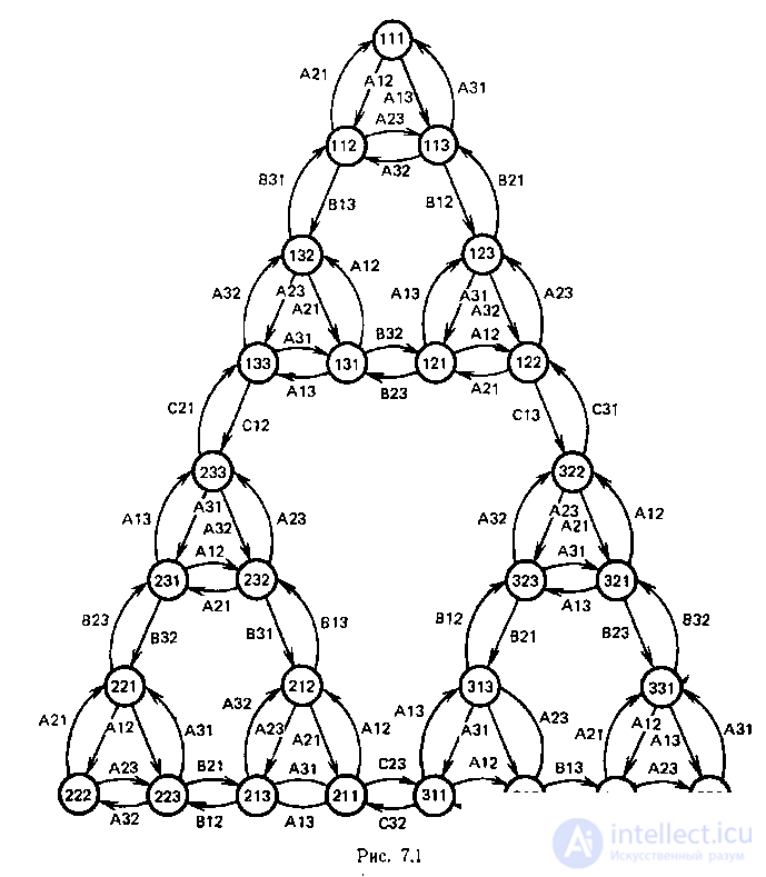
Consider the "Tower of Hanoi" puzzle. There are three pegs 1, 2 and 3 and three disks of different sizes A, B, C with a hole in the center, which can be slipped onto the pegs. In the initial position the disks are on peg 1; the largest disk C is at the bottom and the smallest disk A is at the top. All the disks must be moved to peg 3, moving only one disk at a time. Only the topmost disk on a peg may be taken, and it may not be placed on a disk of smaller size. We use the classical formalization to record the states and the operators. The expression ijk denotes the configuration in which disk C is on peg i, disk B is on peg j and disk A is on peg k. The expression xij denotes the action in which disk x is moved from peg i to peg j. With this formalism all the states and transitions of the puzzle can simply be written as a triangular graph in which the vertices correspond to the arrangements of the disks on the pegs and the arcs to the admissible moves of the disks (Figure 1). This puzzle makes it easy to illustrate all the basic notions of the generalized strategy for problems.
Let us represent the puzzle as an I-problem model. Consider the I-problem R=(B, Γ, P0T), where B={P0, P1,...,P9}; Γ={g }; T=={L 1,L 2,L 3}. The SS-problems P0,P1...,P9 are defined as follows. Figure 1 shows the schema of the SS-problem M==(S, G), where
P0=(S, G, 111, 333), P1=(S, G, 111, 122), P2=(S, G, 122, 322),
P3=(S, G, 322, 333), P4=(S, G, 111, 113), P5,=(S, G, 113, 123),
P6==(S, G, 123, 122), P7=(S, G, 322, 321), P8=(S, G, 321, 331),
P9=(S G, 331,333).
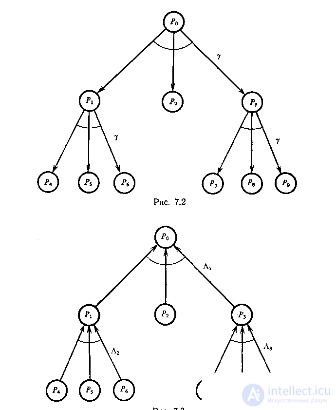
The scheme of the PR-problem N= (B, Γ) is shown in Figure 2; the implicative network T - in Figure 3, where L 1=(P0, P1P2P3, Y ), L 2= (P1, P4P5P6, Y ), L 3== (P3, P7P8P9,Y ), where Y (x1,x2,x3)=x1x2x3.
Problems P2 and P4-P9 are solved by moving a single disk and are elementary. Problems P1 and P3 are solved by manipulating only disks B and A and are simpler than P0. Problems P1 and P3 are solved, whereas problem P0 is reduced to P1, P2 and P3 by a similar manipulation of the disks, whose syntax is expressed by the operator g and whose semantics is expressed by the mapping Y.
Representing this puzzle as a PR-problem (Figure 2) is more compact and more illustrative than representing it as an SS-problem (Figure 1), while representing it as an I-problem (Figure 3) combines the advantages of both and shows the interrelation of the subproblems and of the actions that have to be performed in order to solve the puzzle.
The definitions given above are generalized to the fuzzy case, in which the state of the system for which the problem-solving model is built is not specified exactly and the results of the system's actions
are ambiguous.
In a robotic system, for example, this may be caused by imperfect effectors and receptors and by the limited size of the internal model, which does not reflect the complexity of the surrounding world.
A fuzzy SS-problem is an SS-problem in which i , f are fuzzy sets and the operators g ∈G are fuzzy matrices; an a -solution of a fuzzy SS-problem is a path g=g1...gn,gi∈G,i=1,...,n, such that iOg1O...... OgnOf? a, where O is the max-product of fuzzy matrices.
A fuzzy PR-problem is a PR-problem in which the elements g ∈Γ are assigned a degree of membership m g (p )∈[0,1]; an a -solution of a fuzzy PR-problem is a solution of the PR-problem for which ming ij? a ,g ij ∈yi.
In this case the covering path is called a covering a -path. The degree of membership m g ( p ) is interpreted as the degree of possibility of splitting the problem into subproblems.
A fuzzy implicative scheme is an implicative scheme all of whose mappings Y have a degree of membership m Y ((p )∈[0,1]. The degree of membership is interpreted as the possibility of obtaining a solution of the problem from the solutions of the corresponding subproblems. A fuzzy implicative network is an implicative network with fuzzy implicative schemes. A fuzzy PR-problem represents a fuzzy implicative network if, besides the usual conditions for an implicative network, the following inequality holds: m Y (p )? m g (p ) ? a,
i.e. the possibility of splitting the problem into subproblems is not less than the possibility of obtaining a solution, for every pair of corresponding Y and g.
A fuzzy I-problem is defined in a similar way. However, an a -solution of a fuzzy PR-problem can be built from the a -solutions of its fuzzy subproblems only in particular cases and under additional conditions. Suppose a fuzzy PR-problem is given in which the S are fuzzy SS-problems, and suppose there exists a simplest a -solution Z,
i.e. such a p ∈ S + that m g p ? a , and if p =P1..Pn, then all the problems Pi a -solvable,
where Pi=(Si,Gi,Ji,Fi ). An a -solution of the problem P0 exists when m Y (p )? m g (p )? a for the implicative network. Let us write a more constructive condition for this. Suppose that for every i the operator gi is an a -path solving the problem Pi and Fi=Ji+1. Then, if
max m [Fn∩ (Fn-1∩ (...F1∩ (J o g1)o g2)...)o gn)]? a
and g=g1...gn, then g is an a -solution of the SS-problem P0.
Features of planning goal-directed actions
The further development of planning theory was connected with the construction of "human" models of goal-directed activity. If human reasoning related to planning is viewed as a kind of goal-directed activity aimed at solving intellectual problems, then a planning model must above all take into account the main features of human reasoning.
Suppose some subject world is given in which the action of an intelligent system (IS) consists in reaching goal situations sk from certain initial situations sn by means of action plans; V=bi1...bin, where bi is an executive module from a given set B0. To specify a situation s in such a world means to indicate the properties ci∈ C of the objects ak∈ A0 and the relations between them rp∈ R0 that held, hold or will hold at the moment t. The model of the subject world for such an action of the IS can be represented as Mo=<Ao, Bo, Co, Ro>, and the task of planning actions in the world Mo can be stated as follows: the initial situation sn and the goal situation sk" situations are given, and it is required to build from the executive modules bi∈ Bo an action plan V, which, when applied to Sn, makes it possible to reach Sk.
When solving this task a person usually faces two difficulties. First, as a rule, he has only a vague notion of the particular sk that lies far in the future. He is therefore satisfied with reaching not a particular situation but any situation of the class sk that meets certain requirements. Second, even if he does have a notion of sk, the search for an action plan is still hampered by the high dimensionality of the search space. Thus, an IS needs models of worlds that are more general than Mo.
Among the tasks we single out the class of elementary ones. The rest will be considered complex, and their solutions will be represented as a partially ordered collection of elementary tasks. If the solutions of different complex tasks are similar in some sense, they are generalized. This is how generalized descriptions of tasks of a certain type arise.
From the solutions of elementary tasks the IS builds up the solutions of the complex original tasks. As a rule, however, it cannot find a solution in this way straight away. Standard tasks are therefore used to pass from the original tasks to elementary ones. First, for a given original task the semantic structure of its input data is determined, i.e. a strategic task is posed and a hypothesis of its solution is formed. Then every standard task of the hypothesis is decomposed, which leads to the formulation and solution of tactical tasks and, consequently, to the solution of the original task.
The presence of standard and elementary tasks in the knowledge base indicates a hierarchical structure not only of the knowledge base itself but also of the search procedures; standard tasks may be conditionally assigned to the strategic level of search and elementary ones to the tactical level. The semantic structures of the required results and of the input data of standard tasks are usually revealed as a result of comprehending the required results or the input data of tactical tasks, and are not accessible to direct sensory perception. Thus, at the strategic level every tactical situation (input data or required result) is evaluated by the presence in it of familiar semantic structures. For example, in chess the semantic structures are expressed by the concepts "developed position", "open position", and so on. At the tactical level the system solves the tactical tasks projected down from the strategic level through the decomposition of standard tasks - for example, creating a passed pawn in chess.
Thus, the reasoning of an intelligent system (IS) about action planning rests on structured knowledge and directed heuristic search.
Let C1 be the set obtained by coarsening the properties cO C0, B1 - the set of elementary tasks obtained by renaming the executive modules biO B0, A1 ≤ A and R1≤ Ro. Then the world model of tactical tasks can be represented as Mo=<A1, B1, C1, R1>, and the statement of a tactical task p-
as the pair <sn, sk >, and its solution as the collection V = b1,..., bin. Obviously, owing to the coarsening just described, in the world M1 the individual states of objects and executive modules become indistinguishable. However, such a simplification, caused by the "coarseness" of the sensory organs of the IS, is still not enough to reduce substantially the dimensionality of the solution search space V, and therefore a further generalization of M1 is needed, this time at the conceptual level.
In the world M1 tactical situations s are described, just like the situations s in the world M0, through the properties of objects and the relations between them. Such descriptions, however, are not holistic in character, since they do not contain semantic structures in explicit form. The identification of such generalized structures, and also the formation of the tactical situations s corresponding to them, are carried out on the basis of the concepts available to the IS and amount to its comprehension of the current or goal situations s from the standpoint of these concepts, which in this case are used as test programs. Thus, in the world M2 the situations s in question are represented as aggregated objects ak O A2, whose properties ci O C2 and the relations r2 O R2 between which, like the aggregated objects themselves, are determined by the test concepts. The situation is similar with the solutions V in the world M1. A holistic description of V means describing these solutions precisely as standard tasks. Thus, in the world M2 there are standard tasks bi O B2.
Complexity estimates for the planning problem
Let us present a number of results concerning the complexity of solving planning problems.
1. The analysis of computational problems turns out to be a PSPACE-complete problem even provided that there are no "empty" quantities W.
2. For computational models without functional quantities, i.e. with empty Db and F, the problem of analyzing computational problems turns out to be: a) PSPACE-complete for H containing functional and operator dependencies without W; b) NP-complete for H, containing only functional and variant dependencies without the "empty" quantity W; c) polynomial (in the running time of the planner) for H, containing only functional and implicit dependencies; d) planners with linear running time can be constructed for H with functional dependencies only and without W, and for H with functional and implicit dependencies.
In the PGIZ system Db and F are empty, and H contains only functional and operator dependencies without the "empty" quantity W. The SPORA system for the automatic synthesis of programs uses predicate calculus, for which a special inference strategy has been developed.
An analysis tree for a computational problem is a tree of formulas of the calculus being used, at whose root stands the formula representing the original problem; every non-terminal vertex of the tree can be obtained by one of the inference rules of the "calculus of computational problems" from the formulas located immediately below it in the tree, whereas the terminal (leaf) vertices are not the conclusion of any inference rule of the "calculus of computational problems".
A planner in such a calculus works as follows: for the given problem some analysis tree is constructed. If all of its leaf vertices are axioms, then a program is "assembled" from this tree. Otherwise, a justification is produced that the problem is unsolvable. The absence of determinism in logical inference in calculi of the standard type leads to an exponential enumeration of the possible branches. Detecting a dead end during such an enumeration proves useless (or almost useless) for the search along the other branches of the inference tree. In the "calculus of computational problems" it is sufficient for the planner to have some analysis tree in order to solve the problem completely. Given a sensible strategy for constructing analysis trees, this makes it possible to obtain comparatively fast planning procedures.
In the general case the planner has to solve a PSPACE-complete problem. This means that all planners known at present run in exponential time on almost all computational problems. In reality the situation is not so bad. Problems of practical interest, as a rule, admit efficient planning. And although the fraction of such problems tends to zero as the parameters that define them grow, it is precisely these problems that are of interest from the standpoint of the efficiency of automatic program synthesis. An indicator of practically interesting problems can be the degree of interaction of the subproblems in the course of solving the original problem. The notions of "subproblem" and "subproblem conditions" arise already at the stage of the naive interpretation of the following dependencies.
The functional dependency (F->Y1), where F is a functional quantity of type (X->-Y), which presupposes the prior synthesis of a procedure for computing F, whose input parameters are the quantities from the list X.
Operator dependencies, which presuppose the synthesis of m procedures with inputs that are the "subproblem conditions" X1, X2,..., Xb-
Variant dependencies, which presuppose that two branches of computation are created: for the first one the values of all the quantities from the list Y1, are known, and for the second one those from the list Y2.
Let us consider a simple (but typical) example. Suppose there are a functional dependency D1: (A, B, CR E) and operator dependencies D2: ((CR E ) R E1), D3:(( BR E1))R E2)), D4: ((AR E2 ) R E3). It is required to find E3. To this end one has to solve the subproblem (AR E2 ). If we make use of dependency D3, we arrive at the search for a solution of the new subproblem ( BR E1). If dependency D2, is used, we arrive at the need to solve the subproblem ( CR E), which, according to D1 is solvable only when A and B are known. The degree of interaction of the subproblems in this example equals three. This process is a typical scheme of planning in the space of problems.
For planners operating within the "calculus of computational problems;", the synthesis of a solution to a computational problem takes time hqrl/r!, where h - is a constant, l is the length of the problem specification, defined as the total number of occurrences of the names of the quantities used in F and H, q- is the total number of "distinct" arguments of the quantities taken from the "subproblem conditions" in the operator dependencies from H and from the "variant conditions" in the variant dependencies from H, r-is the minimum degree of interaction among the subproblems of the original problem. This estimate is quasi-optimal in nature. The planner runs for a long time only on problems that are not natural, since such problems require the maximum possible interleaving of all the subproblems into which the original problem is decomposed. Experiments show that for problems encountered in practice the planner's running time is polynomial. The memory required for the planner to operate within the "calculus of computational problems" is estimated as bl2, where b - is a constant. If H contains no variant dependencies, only a linear amount of memory is required, dl, where d-is a constant.
In the planners known today, the programs produced are far from optimal. There is a tendency for program quality to deteriorate as the planner's running time is reduced. Moreover, synthesizing optimal sequential programs is harder than synthesizing optimal parallel programs. In view of the development of computers with a new architecture oriented toward parallel processes, this circumstance may prove advantageous. For example, the problem of finding programs with minimal sequential execution time for solving computational problems in which Db is empty while H consists only of functional dependencies W , turns out to be NP-complete in the strong sense. On the other hand, within the "calculus of computational problems", provided that Dbis empty and H consists of functional and implicit dependencies, it is possible, in linear time kl (k - a constant), to synthesize a program whose parallel execution requires the minimum time achievable for the given problem.
In the PRIZ system and its modifications, a computational problem is considered solvable if the formula corresponding to it is derivable in the positive fragment of the intuitionistic propositional calculus, that is, if and only if the planner of the PRIZ system succeeds. For the "calculus of computational problems", two semantics of solvability are possible.
The extremely non-constructive one; a computational problem is considered solvable if in every database (every interpretation) satisfying all the constraints of the computational model there exists some function of type (XR Y);
the extremely constructive one: a generalized standard program schema is considered a solution of a computational problem if in every interpretation satisfying all the constraints of the computational model there exists a function of type (XR Y), computed by the program P that is obtained from the generalized standard program schema by the corresponding instantiation of the predicate and function symbols.
The "calculus of computational problems" is sound and complete with respect to both semantics. Under the first semantics the planner always delivers a solution of the original problem in the form of a correct program; under the second, the class of all propositional formulas describing solvable computational problems coincides with the class of all formulas derivable in the intuitionistic propositional calculus. This shows that the "calculus of computational problems" may be regarded as one of the ways of formalizing the previously proposed interpretation of intuitionistic logic as a logic of "problems".
Many information systems (IS) employ planners whose capabilities are substantially broader than those of the planner of the PRIZ system or of the one used in the "calculus of computational problems". The calculi that the planners of many computer-aided design, planning and control systems deal with are broader than intuitionistic propositional calculi. They make use of heuristic considerations that have no analogs in the relations in terms of which computational models were described above. An example is the planner of the MAVR system, intended for a computer-aided design IS. During its operation, situations arise that are not solvable within the theory described above. Such cases compel one to look for other ways of building a system for searching for action plans.

Comments