
Lecture 15 min.
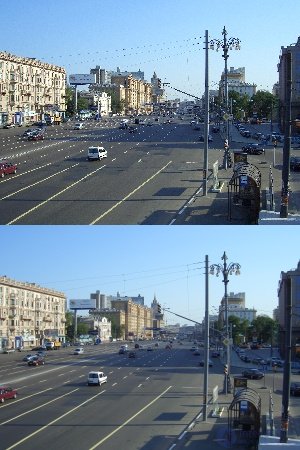
Resampling in signal processing is a change in the sampling rate of a discrete (most often digital) signal. Resampling algorithms are widely used in the processing of audio signals, radio signals, and images (resampling a raster image means changing its resolution in pixels).
The signal samples corresponding to the new sampling rate are computed from the existing samples and contain no new information.
Increasing the sampling rate is called interpolation, and decreasing it is called decimation.
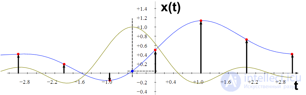
Computing an intermediate sample (at the point −0.5) of a discrete signal using an ideal low-pass filter. The blue curve is the original continuous signal, and the green one is the impulse response of the ideal low-pass filter. For interpolation, the values of the impulse response at the sample points, multiplied by the values of the corresponding samples, are summed.
According to the Nyquist–Shannon (Kotelnikov) sampling theorem, any continuous signal with a finite spectrum (that is, a spectrum in which the spectral components corresponding to frequencies greater than or equal to some frequency  are absent) can be represented as samples of a discrete signal with the sampling rate
  . Moreover, this transformation is one-to-one, that is, if the conditions of the sampling theorem are met, the original signal with a band-limited spectrum can be recovered from the discrete signal without distortion.
In resampling, the samples of a signal corresponding to one sampling rate are computed from the existing samples of the same signal corresponding to another sampling rate (it is assumed that both sampling rates satisfy the conditions of the sampling theorem). Ideal resampling is equivalent to reconstructing the continuous signal from its samples and then sampling it at the new rate.
The value of the original continuous signal at a given point is computed exactly as follows:
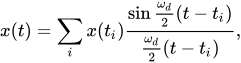
where  is the i-th sample of the signal,
  is the time instant corresponding to this sample,
  is the angular sampling frequency, and
  is the interpolated value of the signal at the time instant
  .
.
The function 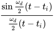 is not finite in extent, so computing the value of the signal at a given instant using the expression above requires processing an infinite number of its samples (both in the past and in the future), which is impossible in practice. In real life, interpolation is performed with other filters, and the expression for it takes the following form:
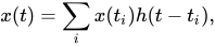
where  is the impulse response of the corresponding reconstruction filter. The type of this filter is chosen depending on the task.
Directly computing new signal samples using the formulas above requires significant computational resources and is undesirable for real-time applications. There are important special cases of resampling for which the new samples are computed more simply:
 ) factor (this case can be viewed as a combination of the previous two).
Under such restrictions, it becomes convenient to use standard digital filter implementations for resampling.
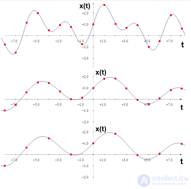
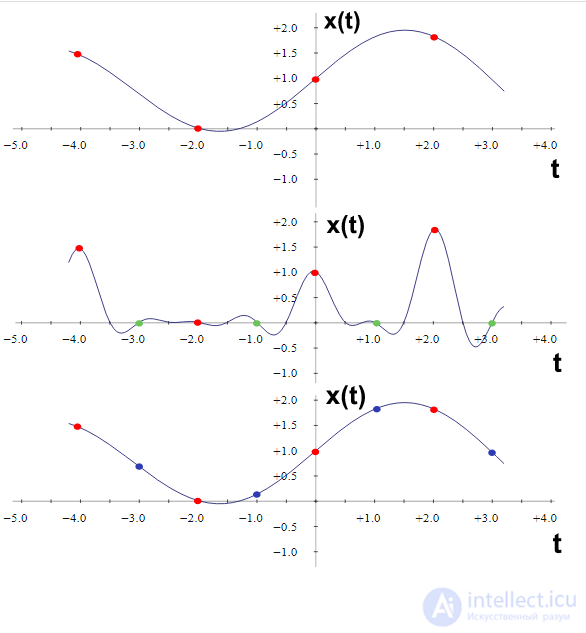
The choice of the function is a compromise between the quality of resampling (that is, how close it is to ideal) and the computational complexity of the process. In principle, any low-pass filter with the required cutoff frequency can be used for resampling. FIR filters are used for these tasks more often than IIR filters because FIR filters can be built with a linear phase response.[10]
The following classes of digital filters are most often used in resampling:[11]
1. Filters designed on the criterion of closeness of the frequency response to that of an ideal low-pass filter:
1.1. Windowed sinc filters, whose impulse response is obtained by multiplying the impulse response of the ideal low-pass filter by a window function,
1.2. Equiripple Chebyshev filters.
2. Classical function interpolation methods (often used for images)[12]:
2.1. Linear interpolators,
2.2. Lagrange interpolators (a special case is cubic interpolation).
3. CIC filters (cascades of comb filters and integrators).[13] This class of filters does not use multiplications in its computation, which saves computational resources.
The process of reducing the sampling rate of a signal is called decimation. Sometimes this term is used only for reducing the sampling rate by an integer factor (hereafter  ).[14] Decimation of a digital signal by an integer factor is performed in two stages:[10][15]
-th sample is kept).In English-language literature, the second of these stages is sometimes denoted by the term downsampling.[16] In everyday usage, this term may be used as a synonym for "decimation".
The first stage is necessary to eliminate aliasing, whose nature is similar to the aliasing that occurs during the initial sampling of an analog signal.[15] Aliasing is especially noticeable in those parts of the signal that contain significant high-frequency spectral components. Thus, in the photographs at the beginning of the article, the sky has practically not been affected by aliasing, but the effect becomes noticeable if you look at the sharp transitions.
When the decimation algorithm is implemented in software, the "extra" samples are not deleted but simply never computed. As a result, the number of calls to the digital filter is reduced by a factor of . In a hardware implementation, savings can be achieved by using polyphase filters.
Interpolation is an increase in the sampling rate by an integer or fractional factor by computing intermediate samples from the existing ones. Ideal interpolation makes it possible to restore the values of the signal at the intermediate samples exactly.
The standard algorithm for interpolating a signal by an integer factor is as follows:
In English-language literature, the first of these steps is sometimes called upsampling. In everyday usage, this term may also be used as a synonym for "interpolation."
In a software implementation of interpolation, the zero samples do not take part in computing the filter output, which makes it possible to optimize the computation. In a hardware implementation, polyphase filters can be used to save resources
To change the sampling rate of a signal by a factor of  (
( and are positive integers), you can first increase the sampling rate by a factor of and then reduce it by a factor of . It is enough to filter the signal just once, between the interpolation and the decimation
The drawback of this method is that the signal has to be filtered at a sampling rate raised by a factor of , which requires significant computational resources. The corresponding rate can be many times higher than both the original and the final resampling rate, especially if and are close large numbers. For example, when resampling an audio signal from 44100 Hz to 48000 Hz by this method, the sampling rate must be increased 160 times to 7056000 Hz and then reduced 147 times to 48000 Hz. Thus, in this example the computations have to be performed at a sampling rate of more than 7 MHz.
The polyphase-filter resampling method is similar to the previous one, except that instead of a single filter running at a high sampling rate, it uses several filters running at a low rate. This reduces the amount of computation required, since for each sample only the output of one of these filters has to be computed
A polyphase filter is a set of small filters working in parallel, each of which processes only a subset of the signal samples (if there are filters in total, each filter will process only every -th sample).
Polyphase filters are used for resampling by both integer and fractional factors
Resampling with the DFT is used to increase the sampling rate by an integer or fractional factor. The algorithm works only with finite segments of a signal. Let be the initial number of samples and the number of samples in the resampled signal. The algorithm includes the following operations:[25][26]
1. The DFT of the original signal is computed (most often with the fast Fourier transform algorithm).
2. The required number of zero components is inserted into the middle of the spectrum:
2.1. if is odd:
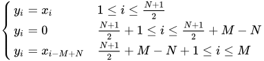
2.2. if is even:
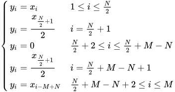
3. The inverse discrete Fourier transform is computed, with normalization.
Any DFT-based method is intended primarily for periodic discrete signals. To process non-periodic signals, the segments used to compute the DFT must be chosen so that their ends overlap.
Both hardware implementations of resampling algorithms (based on specialized chips or FPGAs ) and software implementations (on general-purpose processors (see below) or digital signal processors ) are widely used.
The choice of a particular resampling implementation is the result of a compromise between conversion quality and computational complexity. The main parameter affecting these characteristics is how close the digital filters used are to the ideal ones. Higher-quality filters require more computational resources
In practice, resampling in most cases leads to a loss of information about the signal, for the following reasons:
Thus, if the sampling rate is increased and then reduced back to the original value, the signal quality will be lost (unless the high rate is a multiple of the low one).
Oversampling means sampling a signal at a rate several times higher than the Nyquist (Kotelnikov) rate, followed by decimation. This approach offers the following advantages :
A similar approach is used when reconstructing a signal from its samples, in order to simplify the analog reconstruction filter.
Equipment intended for playing back digital audio is, as a rule, designed for a specific, fixed sampling rate immediately before digital-to-analog conversion. All audio signals with other sampling rates must sooner or later be resampled .
Resampling an audio signal to the required rate can be done by the media player, the sound card driver, or the sound card itself. Using the player software for this purpose can be justified if you want to avoid hardware resampling (or resampling by the driver) in order to achieve higher quality (at the cost of higher CPU load). However, software resampling of the played material to a rate other than the one supported by the hardware makes no sense and only degrades the signal quality.
There are open-source software resamplers for audio signals:
Resampling is also supported by audio editors (such as Adobe Audition, Sony Sound Forge or Audacity).
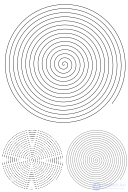
Changing resolution is one of the most common image processing operations. Resampling that comes close to the ideal is not always desirable. On the contrary, the results of filters with a frequency response far from ideal may be perceived visually as good. The choice of a resampling filter is a compromise between the type and severity of artifacts and the computational complexity of the conversion (which matters for real-time applications).
Typical artifacts when changing image resolution:
A large number of filters are used for image resampling, and they can be classified as follows:
The images below illustrate the application of the most commonly used image resizing filters. When an image is enlarged without a filter, it stays sharp but pixelated. With bilinear interpolation, the pixelation is less noticeable, but the image is blurred. With the Gaussian filter, the image is blurred, but there is practically no visible pixelation. With the Lanczos filter, there is no pixelation, the image is also blurred, and ringing is visible (seen as a light halo around the shapes).
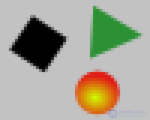
Image enlarged 4 times without a filter

Image enlarged 4 times with bilinear interpolation

Image enlarged 4 times with the Gaussian filter

Image enlarged 4 times with the Lanczos filter
When demodulating digital signals, it is desirable for the sampling rate of the signal to be a multiple of its symbol rate (in other words, for each symbol to correspond to the same number of signal samples). However, the sampling rate of an input signal from an ADC is usually fixed, while the symbol rate may vary. The solution is to resample the signal

Comments