
Lecture
This article examines the atmospheric correction of satellite images using the DOS (Dark Object Subtraction) method. At the end of the article, a ready-made software toolkit for performing atmospheric correction is presented.
Contents
|
The geodata source was USGS (United States Geological Survey) data, available for free download. Data from these resources is provided in GeoTIFF format as continuous sets of scenes for various regions of the world. The geodata provided on these resources corresponds to processing level LG1, "raw geodata" that has not been converted to at-sensor radiance values. For independent conversion and atmospheric correction, satellite sensor configuration files are available with a set of parameters: minimum and maximum pixel brightness in the image; minimum and maximum radiance at the sensors; minimum and maximum reflectance from the earth's surface (Landsat 8); and much more. In addition to the satellite sensor configuration data, the archive contains several GeoTIFF files divided by band number, whose number and composition differ between satellites (Landsat 5, 7 and 8) (Table 1).
Table 1 — Satellites and the bands used in this work
| Satellite and sensor | Band number | Spectrum name | Wavelengths (nm) |
|---|---|---|---|
| Landsat 5 TM | 1 | Blue | 450–520 |
| 2 | Green | 520–600 | |
| 3 | Red | 630–690 | |
| 4 | NIR — Near infrared | 760–900 | |
| 5 | SWIR1 — Shortwave infrared 1 | 1550–1750 | |
| 7 | SWIR2 — Shortwave infrared 2 | 2080–2350 | |
| Landsat 7 ETM+ | 1 | Blue | 450–520 |
| 2 | Green | 520–600 | |
| 3 | Red | 630–690 | |
| 4 | NIR — Near infrared | 770–900 | |
| 5 | SWIR1 — Shortwave infrared 1 | 1550–1750 | |
| 7 | SWIR2 — Shortwave infrared 2 | 2080–2350 | |
| Lansat 8 Oli | 2 | Blue | 450—515 |
| 3 | Green | 525—600 | |
| 4 | Red | 630—680 | |
| 5 | NIR — Near infrared | 845—885 | |
| 6 | SWIR1 — Shortwave infrared 1 | 1560—1660 | |
| 7 | SWIR2 — Shortwave infrared 2 | 2100—2300 |
As the table shows, the six most commonly used "spectra" lie in a similar frequency range on different satellites. Therefore, for convenience of terminology, instead of specifying satellite bands we will hereafter use the names of the spectra themselves: BLUE, GREEN, RED, NIR (near infrared), SWIR1 (shortwave infrared 1), SWIR2 (shortwave infrared 2), regardless of the satellite, and apply the same set of calculations to them.
As already mentioned, the geodata for all bands is provided at processing level LG1, in raw form. This means that the provided band GeoTIFFs are nothing more than brightness "photographs" positioned on the terrain, which in this form cannot be used for GIS research. Therefore, LG1 data must be normalized, that is, the brightness values must be converted to at-sensor radiance and an atmospheric correction must be applied.
The theoretical basis of the conversion process is described in detail in the article "Converting TM and ETM+ data to at-sensor radiance", so we will touch only on the practical implementation of the process.
Conversion is the first stage of normalizing raw geodata and is a mathematical operation that converts the pixel brightness values of a geoimage into values of the radiation received by the satellite sensors. For this conversion, the Landsat data package includes the correction file _MTL.txt, whose limit values are used at this stage of geoimage processing.
For this work we used the standard formula (1), described in the NASA documentation, for converting brightness to top of atmosphere radiance (TOA radiance).
 (1)
(1)
where:
Lλ — spectral radiance received by the satellite sensor;
DNcal — pixel brightness values of the raw geoimage;
Qcalmin — minimum possible pixel value of the geoimage;
Qcalmax — maximum possible pixel value of the geoimage;
LMINλ — minimum spectral radiance value for the particular satellite sensor for the particular image;
LMAXλ — maximum spectral radiance value for the particular satellite sensor for the particular image.
In addition, the simplified formula (2) can be used to calculate TOA radiance (Thome et al., 1994, Lu et al., 2002).
Lλ = DNcal × Gainλ + Baisλ (2)
where:
Lλ — spectral radiance received by the satellite sensor;
DNcal — pixel brightness values of the "raw" geoimage;
Gainλ — radiance gain relative to the brightness of the original geoimage;
Baisλ — radiance offset (bias) relative to the brightness of the original geoimage.
After processing every pixel of the geoimage with this formula, we obtain a matrix of floating-point values, the normalized geodata.
The next stage of geodata normalization is to reduce the influence of the atmosphere on the image and to convert the radiance that reached the satellite sensors (TOA radiance) into values of the solar spectral radiation actually reflected from the ground.
The material in this and the following sections overlaps to some extent with the article "Atmospheric correction of Landsat/ETM+ data (COST method)", but unlike it, it is oriented toward batch processing of remote sensing data from several sources.
The influence of the atmosphere on a geoimage shows up through a number of factors: the angle of incidence and reflection of the sun's rays, atmospheric transparency, the gas factor and haze (Figure 1).
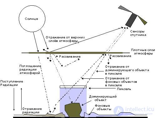
Fig. 1. Factors affecting the arrival of reflected solar radiation at the satellite sensors.
For further research, it is necessary to perform an optical correction (normalization) of the geoimage data using the Dark Object Subtraction (DOS) method, first presented by Chavez (1996). The essence of the method is to find the brightness of the one-percent dark object of the geoimage and then correct the minimum value of every image pixel relative to the spectral brightness of the object found.
There are two main ways to find the 1% dark object (Dark Object) for the DOS method:
In this work, method (2) was applied successfully and performed well when processing a large number of geoimages of the study area.
After determining the brightness of the Dark Object (in later calculations we will denote it DNmin), we perform the atmospheric correction using the DOS method in several stages:
1. Calculate the radiance corresponding to the brightness of the 1% dark object (the calculation is performed by analogy with TOA radiance), using formula (3).
 (3)
(3)
where:
Lλmin - spectral radiance for the 1% dark object;
DNmin - pixel brightness value of the 1% dark object;
Qcalmin - minimum possible pixel value of the geoimage;
Qcalmax - maximum possible pixel value of the geoimage;
LMINλ - minimum spectral radiance value for the particular satellite sensor for the particular image;
LMAXλ - maximum spectral radiance value for the particular satellite sensor for the particular image.
Or using the simplified form (4).
Lλmin = DNmin × Gainλ + Baisλ (4)
where:
Lλmin - spectral radiance for the 1% dark object;
DNmin - pixel brightness value of the 1% dark object;
Gainλ - radiance gain relative to the brightness of the 1% dark object;
Baisλ - radiance offset (bias) relative to the brightness of the 1% dark object.
2. Calculate the coefficient of the influence of the angle of incidence and reflection of the sun's rays for the 1% dark object using formula (5).
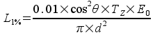 (5)
(5)
where:
L1% - coefficient of the influence of the angle of incidence and reflection of the sun's rays for the 1% dark object;
d - Sun-Earth distance in astronomical units on the specific day the scene was acquired over the specific area ;
E0 - coefficient of solar exo-atmospheric spectral irradiance (given explicitly as tabulated data and taken into account in the calibration of the Landsat 5 and 7 sensors; for Landsat 8 it is calculated additionally);
θ - solar zenith angle in radians;
TZ - measure of the transmittance of radiation from the sun to the earth; in the DOS2 method it is taken to be cosθ.
3. Calculate the atmospheric haze value (hazing) using formula (6).
Lλhaze = Lλmin - L1% (6)
where:
Lλhaze — atmospheric haze value (hazing);
L1% — coefficient of the influence of the angle of incidence and reflection of the sun's rays for the 1% dark object;
Lλmin — spectral radiance for the 1% dark object.
4. Calculate the atmospherically corrected values of reflected solar radiation using formula (7)
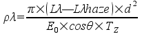 (7)
(7)
where:
ρλ — atmospherically corrected values of reflected solar radiation;
Lλ — radiance values received by the satellite sensor;
Lλhaze — atmospheric haze value (hazing);
d — Sun-Earth distance in astronomical units on the specific day the scene was acquired over the specific area ;
E0 — coefficient of solar exo-atmospheric spectral irradiance (given explicitly as tabulated data and taken into account in the calibration of the Landsat 5 and 7 sensors; for Landsat 8 it is calculated additionally);
θ — solar zenith angle in radians;
TZ — measure of the transmittance of radiation from the sun to the earth; in the DOS2 method it is taken to be cosθ.
If some of the scenes were acquired by the Landsat 8 satellite (OLI sensor), they must be compared with scenes from Landsat 5 (TM sensor) and Landsat 7 (ETM+ sensor). In this context, a known problem is the application of standard atmospheric correction methods to the new satellite: the calibration of the Landsat 8 OLI sensors is performed without the coefficient of solar exo-atmospheric spectral irradiance Eo (Sobrino et al., 2004) or, as it is called in other sources, Esun. Instead of this coefficient, some new spectral parameters were added to the _MTL.txt correction file: REFLECTANCE_MULT_BAND, the reflectance gain, and REFLECTANCE_ADD_BAND, the reflectance offset, for each of the spectral sensors. As a result, according to the intent of the authors of the changes, the TOA reflectance for Landsat 8 should be calculated using formula (8).
ρλ' = MρQcal+ Aρ (8)
where:
ρλ' — top-of-atmosphere planetary reflectance (TOA reflectance), without correction for the angle of incidence and reflection of the sun's rays;
Mρ — band-specific multiplicative rescaling factor (REFLECTANCE_MULT_BAND_x, where x is the band number) — the reflectance gain;
Aρ — band-specific additive rescaling factor (REFLECTANCE_ADD_BAND_x, where x is the band number) — the reflectance offset;
Qcal — pixel brightness values of the "raw" geoimage (DN).
The TOA reflectance corrected for the angle of incidence and reflection of the sun's rays is calculated using formula (9).
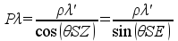 (9)
(9)
where:
ρλ — top-of-atmosphere planetary reflectance (TOA reflectance), with correction for the angle of incidence and reflection of the sun's rays;
θSE — sun elevation above the horizon. Available in the _MTL.txt file in the parameter (SUN_ELEVATION);
θSZ — solar zenith angle; θSZ = 90° - θSE.
The developer community of the free GIS GRASS points to identical REFLECTANCE_MULT_BAND and REFLECTANCE_ADD_BAND values for all bands of the image , which cannot be the case in reality. In its normalization and atmospheric correction module i.landsat.toar, this group applies to rasters acquired by Landsat 8 OLI sensors the same mathematical methods as for Landsat 5 TM and Landsat 7 ETM+, and calculates the missing coefficient Eo (Esun) using formula (10).
 (10)
(10)
where:
Esun — (E0) the calculated coefficient of solar exo-atmospheric spectral irradiance;
d — Sun-Earth distance in astronomical units on the specific day the scene was acquired over the specific area ;
RADIANCE_MAXIMUM — band-specific multiplicative rescaling factor (RADIANCE_MAXIMUM_x, where x is the band number) — the maximum possible value of the radiance reaching the sensor;
REFLECTANCE_MAXIMUM — band-specific multiplicative rescaling factor (REFLECTANCE_MAXIMUM_x, where x is the band number) — the maximum value of the radiation reflected from the earth's surface.
Another peculiarity of Landsat 8 is the reduced sensitivity of the RED, NIR and SWIR1 bands relative to Landsat 7 and 5, which leads to changes in the values of indices calculated from these spectra.
Neil Flood (2014) tried to solve this problem by introducing additional coefficients, calculated empirically for each band of the geoimage. As a result, the conversion of Landsat 8 TOA reflectance values to values for the same region and the same spectra of Landsat 7 takes the form of formula (11).
ρETM+ = c0 + c1 × ρOLI (11)
where:
ρETM — result of converting the TOA reflectance value from Landsat 8 to Landsat 7;
ρOLI — TOA reflectance value calculated for Landsat 8;
c0 — offset of the reflected radiation between the OLI and ETM+ sensors;
c1 — gain of the reflected radiation between the OLI and ETM+ sensors.
The values of c0 and c1 in formula (11) were compiled by the author into correction tables, which makes it possible to apply them without repeating the calculations presented in the article by Neil Flood, 2014 .
All calculations were performed using the Python programming language. For this purpose, a geodata normalization program was written using the GDAL software library, which is closely tied to the numpy extension, which adds to Python support for large multidimensional arrays and matrices, as well as a set of low-level mathematical functions for operating on them. The program consists of the following structural elements:
The program source code is available for download here: https://github.com/oldbay/raster_tools, and the original GeoTIFF rasters and the normalized spectral rasters are available here: https://github.com/oldbay/paper_examples

Comments