
Lecture 2 min.
Grid-based heatmap
Divides the area of interest into a uniform grid of cells.
Each cell stores the counts or statistics of the points that fall inside it.
Provides precise, discrete aggregation that is useful for quantitative analysis.
Example: the number of wildfires per 1 km² cell.
The resolution can be adjusted by changing the cell size.
Binned heatmap
Groups data into bins but visualizes density as a continuous surface .
Shows relative intensity (hot and cold spots) rather than exact counts.
Useful for quick pattern recognition and density visualization.
Example: the density of wildfires across Texas, shown as smooth gradients.
| Feature | Grid-based heatmap | Binned heatmap |
|---|---|---|
| Aggregation | Counts/statistics for each uniform cell | Density represented as a continuous surface. |
| Precision | High (exact counts per cell) | Lower (relative density only) |
| Use case | Analytical tasks, quantitative comparisons | Quick visualization, pattern detection |
| Resolution | Adjustable via cell size | Adapts dynamically to zoom |
| Boundaries | Explicitly defined grid boundaries | No strict boundaries, smooth gradients. |
| Example | Number of fires per km² | High-intensity fire hotspots |
Grid-based approaches often use spatial indexing (quadtrees, rasterization) to efficiently count the points in each cell.
Binned heatmaps use kernel density estimation (KDE) or Gaussian smoothing to interpolate density across space.
In a three-dimensional context, grid heatmaps can represent latent variables in a cubic space, for example the shortest distances between grid points and object skeletons for keypoint detection.
Choose grid-based heatmaps when:
You need exact data/statistics .
You want to compare uniform spatial units.
Analytical rigor is required (for example, in epidemiology or resource allocation).
Choose binned heatmaps when:
You need a quick visualization of density.
Patterns matter more than exact numbers.
The goal is exploratory analysis or presentation.
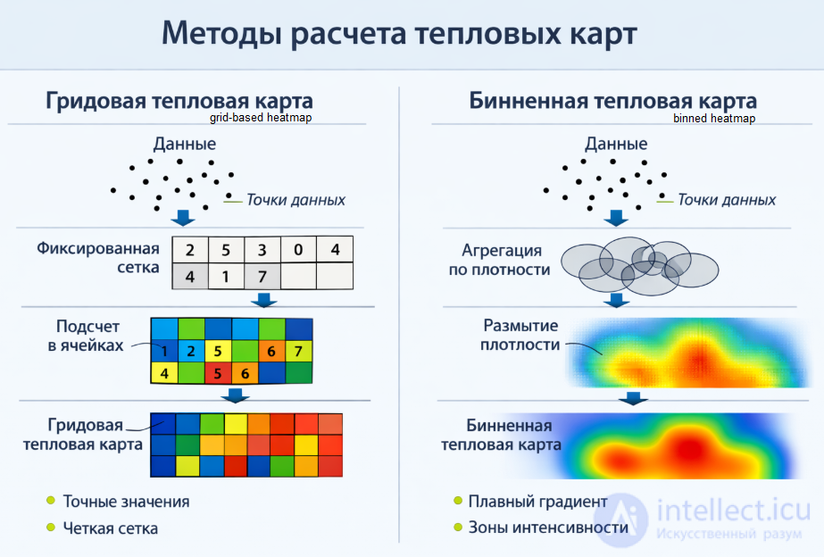
Figure: a schematic example of heatmap computation: left, grid-based (cells with exact counts); right, binned (smooth density gradient).
It demonstrates two approaches:
Grid heatmap — a fixed grid with points counted in each cell; the result is a discrete map with colored squares.
Binned heatmap — density smoothing; the result is a smooth gradient showing zones of intensity.
Thus it is clear at a glance: the first gives exact values per cell, the second gives the overall picture of the distribution.

Comments